Approximate Filters for State Estimation · Principles of Robot Autonomy

In Chapter 11, we introduced the Bayes filter as the canonical framework for state estimation. The Bayes filter uses a recursive procedure that alternates between prediction, using a probabilistic state transition model, and correction, using a probabilistic measurement model. Intuitively, the prediction step answers the question, “Where do we expect to be now, given where we were and how we moved?”, while the correction step asks, “How should we revise that expectation in light of the new sensor data?”

While conceptually elegant, the Bayes filter is rarely tractable to implement in its full generality. The integrals in the prediction step and the normalization in the correction step can be computationally intractable for continuous, high-dimensional state spaces. In discrete domains, exact enumeration is possible in principle but becomes impractical as the number of states grows. As a result, practical state estimation algorithms rely on approximations of the belief distribution. Over time, two broad families of approximations have emerged:

•

Parametric filters: parametric filters assume that the belief distribution belongs to a specific parametric family (most commonly Gaussian), characterized by a fixed set of parameters such as mean and covariance ⁷7. Thrun, S., Burgard, W., Fox, D. Probabilistic Robotics. MIT Press, 2005.. By exploiting the structure of this representation, the belief can be updated efficiently at each time step. The Kalman filter and its variants, including the extended Kalman filter and unscented Kalman filter, are prominent examples.
•

Non-parametric filters: non-parametric filters do not assume a fixed functional form for the belief distribution. Instead, the distribution is approximated directly, either through discretization as in histogram filters or through sampling as in particle filters. This flexibility allows non-parametric methods to represent multimodal and highly irregular belief distributions, although often at a higher computational cost.

Viewed together, parametric and non-parametric filters represent two ends of a spectrum. Parametric filters trade representational flexibility for computational efficiency, while non-parametric filters trade efficiency for expressiveness. In robotics practice, both families play a critical role. Parametric filters often suffice when the problem structure is close to Gaussian and unimodal, while non-parametric filters are indispensable when ambiguity, multimodality, or strong nonlinearities are present. It is helpful to view them as complementary rather than mutually exclusive. Many systems use non-parametric methods for global reasoning, then switch to parametric filters for fast local tracking once a unique hypothesis has been identified. For instance, imagine a mobile robot navigating a building. Early in the mission, it may be unsure which corridor or even which floor it is on. In this case, its belief is naturally multimodal and non-parametric methods shine. As the robot gathers more information and locks onto a unique hypothesis, its uncertainty becomes locally well-approximated by a single Gaussian, and parametric filters become attractive for their speed and simplicity.

In the remainder of this chapter, we develop both approaches within a unified narrative. We begin by reviewing the Gaussian distribution in Section 12.1, which forms the foundation of parametric filters. We then introduce the Kalman filter and its variants in Section 12.2 and Section 12.3, which are the most widely used parametric filters in robotics. Next, we turn to non-parametric filters in Section 12.4, where we relax these assumptions and represent beliefs more directly through discretization (Section 12.4.1) or sampling (Section 12.4.2).

12.1 The Gaussian Distribution

Before we introduce specific filters, it is worth pausing to review the Gaussian distribution, which is the workhorse of parametric state estimation. The Gaussian distribution^†^†margin: Also referred to as the Normal distribution. is one of the most widely used probability distributions in science and engineering and plays a central role in robotics state estimation. Its importance arises not only from its frequent appearance in natural noise processes, but also from its favorable mathematical properties that make recursive filtering tractable.

Informally, in one dimension, a Gaussian distribution resembles the familiar “bell curve”: it is centered at its mean, $\mu$ , and its spread is controlled by its variance, $\sigma^{2}$ . In higher dimensions, a Gaussian describes an ellipsoidal cloud of probability mass in the state space. It is high near the mean, low far away, and its covariance matrix tells us in which directions the uncertainty is large or small.

Univariate case.

The probability density function of a one-dimensional^†^†margin: We refer to a one-dimensional Gaussian as univariate and to higher-dimensional cases as multivariate. Gaussian random variable $X$ with mean $\mu$ and variance $\sigma^{2}$ is:

p(x)=\frac{1}{\sqrt{2\pi\sigma^{2}}}\exp\!\left(-\tfrac{1}{2}\tfrac{(x-\mu)^{2% }}{\sigma^{2}}\right).

(12.1)

We write this compactly as $X\sim\mathcal{N}(\mu,\sigma^{2})$ , and say that “ $X$ is distributed as a Gaussian with mean $\mu$ and variance $\sigma^{2}$ ”. The mean, $\mu$ indicates the center of mass of the distribution, and the variance, $\sigma^{2}$ , measures how spread out the distribution is around that center.

Multivariate case.

For an $n$ -dimensional random vector $\bm{X}\in\mathbb{R}^{n}$ with mean $\bm{\mu}\in\mathbb{R}^{n}$ and covariance matrix $\Sigma\in\mathbb{R}^{n\times n}$ , the multivariate Gaussian distribution is defined by:

p(\bm{x})=\frac{1}{\sqrt{\det(2\pi\Sigma)}}\exp\!\left(-\tfrac{1}{2}(\bm{x}-% \bm{\mu})^{\top}\Sigma^{-1}(\bm{x}-\bm{\mu})\right),

(12.2)

and we compactly write $\bm{X}\sim\mathcal{N}(\bm{\mu},\Sigma)$ . The covariance $\Sigma$ captures both the spread of each component of $\bm{x}$ and their pairwise correlations. Geometrically, the level sets of a multivariate Gaussian^†^†margin: Each level set contains points of equal probability density. are ellipsoids centered at $\bm{\mu}$ , with shape and orientation determined by the covariance matrix $\Sigma$ .

The Gaussian distribution exhibits several important mathematical properties related to affine transformations, addition, and multiplication, which make it particularly attractive for use in filtering algorithms. We highlight three that will be used repeatedly in what follows.

Affine transformations.

The first useful property of the Gaussian distribution is that an affine transformation of a Gaussian random variable is also a Gaussian random variable. If the random vector $\bm{X}$ has a multivariate Gaussian distribution with mean $\bm{\mu}$ and covariance $\Sigma$ , then the random variable $\bm{Y}$ computed from an affine transformation:

\bm{Y}=A\bm{X}+b,

also has a multivariate Gaussian distribution with mean $A\bm{\mu}+b$ and covariance $A\Sigma A^{\top}$ . In other words, if $\bm{X}\sim\mathcal{N}(\bm{\mu},\Sigma)$ , then $\bm{Y}\sim\mathcal{N}(A\bm{\mu}+b,A\Sigma A^{\top})$ .

In the context of robotics, this tells us that if our belief over the current state is Gaussian and the dynamics are linear with additive Gaussian noise, then the predicted state is also Gaussian. We can therefore keep track of just the mean and covariance instead of an entire arbitrary density.

Sum.

The next useful property of Gaussians is that the sum of two independent Gaussian random variables is also a Gaussian random variable. Suppose $\bm{X}_{1}$ and $\bm{X}_{2}$ have multivariate Gaussian distributions with means $\bm{\mu}_{1}$ and $\bm{\mu}_{2}$ and covariances $\Sigma_{1}$ and $\Sigma_{2}$ . Then, the random variable $\bm{Y}$ computed by the sum:

\bm{Y}=\bm{X}_{1}+\bm{X}_{2},

also has a multivariate Gaussian distribution with mean $\bm{\mu}_{1}+\bm{\mu}_{2}$ and covariance $\Sigma_{1}+\Sigma_{2}$ . In other words, if $\bm{X}_{1}\sim\mathcal{N}(\bm{\mu}_{1},\Sigma_{1})$ and $\bm{X}_{2}\sim\mathcal{N}(\bm{\mu}_{2},\Sigma_{2})$ , then $\bm{Y}\sim\mathcal{N}(\bm{\mu}_{1}+\bm{\mu}_{2},\Sigma_{1}+\Sigma_{2})$ .

In robotics, this property commonly appears when modeling additive noise. For example, if a robot’s predicted state is Gaussian and we add independent Gaussian process noise, the resulting state distribution remains Gaussian with covariance equal to the sum of the individual covariances.

Product.

The product of two Gaussian probability density functions is also a Gaussian probability density function. Consider two Gaussian probability density functions:

\begin{split}p_{1}(\bm{x})&=\frac{1}{\sqrt{\det(2\pi\Sigma_{1})}}\exp\big{(}-% \frac{1}{2}(\bm{x}-\bm{\mu}_{1})^{\top}\Sigma_{1}^{-1}(\bm{x}-\bm{\mu}_{1})% \big{)}\\ p_{2}(\bm{x})&=\frac{1}{\sqrt{\det(2\pi\Sigma_{2})}}\exp\big{(}-\frac{1}{2}(% \bm{x}-\bm{\mu}_{2})^{\top}\Sigma_{2}^{-1}(\bm{x}-\bm{\mu}_{2})\big{)}.\end{split}

Their product is:

\begin{split}p(\bm{x})&=p_{1}(\bm{x})\cdot p_{2}(\bm{x})\\ &=\frac{\exp\big{(}-\frac{1}{2}(\bm{x}-\bm{\mu}_{1})^{\top}\Sigma_{1}^{-1}(\bm% {x}-\bm{\mu}_{1})-\frac{1}{2}(\bm{x}-\bm{\mu}_{2})^{\top}\Sigma_{2}^{-1}(\bm{x% }-\bm{\mu}_{2})\big{)}}{(2\pi)^{d}\sqrt{\det(\Sigma_{1})}\sqrt{\det(\Sigma_{2}% )}}\\ &=\frac{\exp\big{(}-\frac{1}{2}(\bm{x}-\bm{\mu})^{\top}\Sigma^{-1}(\bm{x}-\bm{% \mu})\big{)}\exp\big{(}-\frac{1}{2}(\bm{\mu}_{1}^{\top}\Sigma_{1}^{-1}\bm{\mu}% _{1}+\bm{\mu}_{2}^{\top}\Sigma_{2}^{-1}\bm{\mu}_{2}-\bm{\mu}^{\top}\Sigma^{-1}% \bm{\mu})\big{)}}{(2\pi)^{d}\sqrt{\det(\Sigma_{1})}\sqrt{\det(\Sigma_{2})}},% \end{split}

where $d$ is the dimension of the covariance matrices, and we can see that the second exponential is constant with respect to $\bm{x}$ . Therefore, the product is a Gaussian probability density function with mean $\bm{\mu}$ and covariance $\Sigma$ :

\begin{split}\Sigma&=(\Sigma_{1}^{-1}+\Sigma_{2}^{-1})^{-1},\\ \bm{\mu}&=\Sigma(\Sigma_{1}^{-1}\bm{\mu}_{1}+\Sigma_{2}^{-1}\bm{\mu}_{2}).\end% {split}

This property underlies the Bayes filter measurement update, where multiplying a Gaussian prior by a Gaussian likelihood yields a Gaussian posterior. The update simply shifts the mean and shrinks or expands the covariance according to how informative and reliable the measurement is.

Why Gaussians in filtering?

These properties ensure that when both the transition and measurement models are linear with Gaussian noise, the Bayes filter reduces to simple recursive updates of the mean and covariance. This leads directly to the family of Kalman filters, which we will introduce in the next section. From a computational point of view, this is extremely attractive. Instead of carrying around an entire function $p(\bm{x}_{t})$ , we only need to carry a vector $\bm{\mu}_{t}$ and a matrix $\Sigma_{t}$ and update them at each time step.

12.2 Kalman Filter

The Kalman filter is the canonical parametric realization of the Bayes filter for systems with linear dynamics and Gaussian noise. Specifically, the Kalman filter uses a multivariate Gaussian distribution to parameterize the belief distribution over possible states. In other words, we assume $\bm{x}_{t}\sim\mathcal{N}(\bm{\mu}_{t},\Sigma_{t})$ , so that:

\text{bel}(\bm{x}_{t})=\frac{1}{\sqrt{\det(2\pi\Sigma_{t})}}\exp\big{(}-\frac{% 1}{2}(\bm{x}_{t}-\bm{\mu}_{t})^{\top}\Sigma_{t}^{-1}(\bm{x}_{t}-\bm{\mu}_{t})% \big{)}.

Example 12.2.1 (Constant-velocity motion in one dimension).

Consider a robot moving along a straight corridor. The state encodes position and velocity:

\bm{x}_{t}=\begin{bmatrix}p_{t}\\ v_{t}\end{bmatrix},

and the robot receives noisy position measurements from a range sensor. A common linear-Gaussian model is:

	$\displaystyle\bm{x}_{t}$	$\displaystyle=A_{t}\bm{x}_{t-1}+B_{t}\bm{u}_{t}+\bm{\epsilon}_{t},$
	$\displaystyle\bm{z}_{t}$	$\displaystyle=C_{t}\bm{x}_{t}+\bm{\delta}_{t},$

where:

A_{t}=\begin{bmatrix}1&\Delta t\\ 0&1\end{bmatrix},\quad B_{t}=\begin{bmatrix}\tfrac{1}{2}\Delta t^{2}\\ \Delta t\end{bmatrix},\quad C_{t}=\begin{bmatrix}1&0\end{bmatrix},

and where the random variables $\bm{\epsilon}_{t}\sim\mathcal{N}(0,Q_{t})$ , $\bm{\delta}_{t}\sim\mathcal{N}(0,R_{t})$ model process noise and measurement noise, respectively. In this setting, the Kalman filter provides the optimal recursive estimator of $\bm{x}_{t}$ in the mean-squared error sense.

Like the Bayes filter, the Kalman filter is split up into two steps, a prediction step and measurement update step. Both steps update the mean $\bm{\mu}$ and covariance $\Sigma$ of the Gaussian belief and rely on several structural assumptions about the system.

We first assume that the initial belief $\text{bel}(\bm{x}_{0})$ is Gaussian with $\bm{x}_{0}\sim\mathcal{N}(\bm{\mu}_{0},\Sigma_{0})$ . We also assume that the state transition model is linear and evolves according to:

\bm{x}_{t}=A_{t}\bm{x}_{t-1}+B_{t}\bm{u}_{t}+\bm{\epsilon}_{t},

(12.3)

where $\bm{x}_{t-1}$ denotes the previous state, $\bm{u}_{t}$ is the current control input, $\bm{\epsilon}_{t}$ is an independent process noise that is normally distributed according to $\bm{\epsilon}_{t}\sim\mathcal{N}(\bm{0},Q_{t})$ , and $A_{t}$ and $B_{t}$ are time-varying matrices that define the dynamics. The matrix $Q_{t}\in\mathbb{R}^{n\times n}$ is the process noise covariance and captures uncertainty in the motion model^†^†margin: Examples include unmodeled accelerations and environmental disturbances.

The affine structure of the dynamics together with Gaussian noise ensures that the distribution of the next state remains Gaussian. That is, if $\bm{x}_{t-1}$ is Gaussian, then $\bm{x}_{t}$ is also Gaussian. The corresponding probabilistic transition model can therefore be written as:

\begin{split}p(\bm{x}_{t}&\mid\bm{x}_{t-1},\bm{u}_{t})=\\ &\frac{1}{\sqrt{\det(2\pi Q_{t})}}\exp\big{(}-\frac{1}{2}(\bm{x}_{t}-A_{t}\bm{% x}_{t-1}-B_{t}\bm{u}_{t})^{\top}Q_{t}^{-1}(\bm{x}_{t}-A_{t}\bm{x}_{t-1}-B_{t}% \bm{u}_{t})\big{)},\end{split}

and therefore the next state is normally distributed with:

\bm{x}_{t}\sim\mathcal{N}(A_{t}\bm{x}_{t-1}+B_{t}\bm{u}_{t},\>Q_{t}).

We also assume that the measurement model is linear and of the form:

\bm{z}_{t}=C_{t}\bm{x}_{t}+\bm{\delta}_{t},

(12.4)

where $\bm{\delta}_{t}$ is an independent measurement noise that is normally distributed according to $\bm{\delta}_{t}\sim\mathcal{N}(\bm{0},R_{t})$ , and $C_{t}$ is a time-varying matrix that defines how the state maps to measurements. The matrix $R_{t}\in\mathbb{R}^{m\times m}$ is the measurement noise covariance that describes the uncertainty in the sensor measurements.

Under these assumptions, the probabilistic measurement model can be expressed as:

p(\bm{z}_{t}\mid\bm{x}_{t})=\frac{1}{\sqrt{\det(2\pi R_{t})}}\exp\big{(}-\frac% {1}{2}(\bm{z}_{t}-C_{t}\bm{x}_{t})^{\top}R_{t}^{-1}(\bm{z}_{t}-C_{t}\bm{x}_{t}% )\big{)},

which implies that $\bm{z}_{t}\mid\bm{x}_{t}\sim\mathcal{N}(C_{t}\bm{x}_{t},\>R_{t})$ . In many robotics applications, the matrix $C_{t}$ selects a subset of the state variables. For example a sensor may measure position but not velocity.

To summarize, the Kalman filter assumes that the initial belief is Gaussian and that both the state transition model and measurement model are linear with additive Gaussian noise. These assumptions guarantee that the belief distribution remains Gaussian after each prediction and measurement update. As a result, the algorithm only needs to propagate the mean $\bm{\mu}$ and covariance $\Sigma$ rather than a full probability distribution. Therefore, while this property makes the Kalman filter computationally efficient, it also limits its applicability to systems that satisfy the assumptions of linearity and Gaussian noise.

12.2.1 Algorithm (Predict–Correct Form)

For clarity, we distinguish between the predicted belief, obtained after applying the control but before incorporating the new measurement, and the corrected belief, obtained after the measurement update. Algorithm 1 details the full algorithm, where we denote the predicted mean and covariance by $\bar{\mu}_{t}$ and $\bar{\Sigma}_{t}$ .

Data:

\bm{\mu}_{t-1},\,\Sigma_{t-1},\,\bm{u}_{t},\,\bm{z}_{t}

Result:

\bm{\mu}_{t},\,\Sigma_{t}

// Prediction (motion update)

\bar{\bm{\mu}}_{t}\;\leftarrow\;A_{t}\,\bm{\mu}_{t-1}+B_{t}\,\bm{u}_{t}

\bar{\Sigma}_{t}\;\leftarrow\;A_{t}\,\Sigma_{t-1}A_{t}^{\top}+\,Q_{t}

// Innovation (measurement residual)

\tilde{\bm{z}}_{t}\;\leftarrow\;\bm{z}_{t}-C_{t}\,\bar{\bm{\mu}}_{t}

S_{t}\;\leftarrow\;C_{t}\,\bar{\Sigma}_{t}\,C_{t}^{\top}+R_{t}

// Kalman gain

K_{t}\;\leftarrow\;\bar{\Sigma}_{t}\,C_{t}^{\top}\,S_{t}^{-1}

// Correction (measurement update)

\bm{\mu}_{t}\;\leftarrow\;\bar{\bm{\mu}}_{t}+K_{t}\,\tilde{\bm{z}}_{t}

// Covariance update (Joseph form for numerical stability)

\Sigma_{t}\;\leftarrow\;(I-K_{t}C_{t})\,\bar{\Sigma}_{t}\,(I-K_{t}C_{t})^{\top%}+K_{t}\,R_{t}\,K_{t}^{\top}

return

\bm{\mu}_{t},\,\Sigma_{t}

Algorithm 1 Kalman Filter (linear-Gaussian)

Intuition.

The Kalman filter can be understood as a repeated negotiation between the model prediction and the sensor measurement. The prediction step propagates the belief through the system dynamics while adding process uncertainty. The measurement update then adjusts this prediction using the newly observed measurement, where the amount of adjustment depends on how reliable the model prediction and the sensor reading are relative to one another. Specifically, the residual $\tilde{\bm{z}}_{t}$ measures the discrepancy between the predicted measurement and the actual observation. The matrix $S_{t}$ describes the expected uncertainty of this residual and is known as the innovation covariance. The Kalman gain $K_{t}$ determines how strongly the estimate should respond to the measurement: when sensor noise is large, $K_{t}$ becomes small and the filter relies more heavily on the prediction; when the model uncertainty is large but the sensor is precise, $K_{t}$ increases and the estimate is pulled more strongly toward the measurement.

12.2.2 Derivation

One way to derive the Kalman filter algorithm is by explicitly evaluating the Bayes filter updates from Chapter 11 with the Gaussian belief structure and probabilistic transition and measurement models. This would involve explicitly computing an integral of $p(\bm{x}_{t}\mid\bm{x}_{t-1},\>\bm{u}_{t})p(\bm{x}_{t-1})$ for the prediction step. Instead, we consider a more intuitive approach that directly leverages the properties of Gaussians presented in Section 12.1 to show that the familiar update equations in Algorithm 1 are an exact consequence of the linear-Gaussian assumptions.

First, from the prior belief distribution, $\text{bel}(\bm{x}_{t-1})\sim\mathcal{N}(\bm{\mu}_{t-1},\Sigma_{t-1})$ , we compute the predicted belief, $\overline{\text{bel}}(\bm{x}_{t-1})$ , by using the affine transformation property of Gaussian random variables and the property concerning the sum of two independent Gaussian random variables. Specifically, we apply these properties to the linear state transition model in Equation 12.3 to give the predicted mean:

\begin{split}\bar{\bm{\mu}}_{t}&=A_{t}\bm{\mu}_{t-1}+B_{t}\bm{u}_{t}+\bm{0},\\ \end{split}

where the $\bm{0}$ comes from the mean of the independent Gaussian process noise, $\bm{\epsilon}_{t}\sim\mathcal{N}(\bm{0},Q_{t})$ . The predicted covariance is then:

\begin{split}\bar{\Sigma}_{t}&=A_{t}\Sigma_{t-1}A_{t}^{\top}+Q_{t}.\\ \end{split}

For the measurement update step of the Bayes filter, we have:

\begin{split}\text{bel}(\bm{x}_{t})\propto p(\bm{z}_{t}\mid\bm{x}_{t})% \overline{\text{bel}}(\bm{x}_{t}),\\ \end{split}

where $p(\bm{z}_{t}\mid\bm{x}_{t})\sim\mathcal{N}(C_{t}\bm{x}_{t},\>R_{t})$ and $\overline{\text{bel}}(\bm{x}_{t})\sim\mathcal{N}(\bar{\bm{\mu}}_{t},\>\bar{% \Sigma}_{t})$ . We can therefore use the fact that the product of two Gaussians probability density functions is also a Gaussian probability density function to compute:

\begin{split}\text{bel}(\bm{x}_{t})=\eta\>\exp\big{(}-\frac{1}{2}J_{t}\big{)},% \end{split}

where $\eta$ is a normalization constant and:

J_{t}=(\bm{z}_{t}-C_{t}\bm{x}_{t})^{\top}R_{t}^{-1}(\bm{z}_{t}-C_{t}\bm{x}_{t}% )+(\bm{x}_{t}-\bar{\bm{\mu}}_{t})^{\top}\bar{\Sigma}_{t}^{-1}(\bm{x}_{t}-\bar{% \bm{\mu}}_{t}).

We compute the mean, $\bm{\mu}_{t}$ , for this new probability density function by finding where the first derivative of $\text{bel}(\bm{x}_{t})$ with respect to $\bm{x}_{t}$ is zero, which occurs when the derivative of $J_{t}$ with respect to $\bm{x}_{t}$ is zero. Similarly, we compute the new covariance, $\Sigma_{t}$ , as the inverse of the second derivative of $J_{t}$ with respect to $\bm{x}_{t}$ . Therefore, we have the conditions:

\begin{split}0&=-C_{t}^{\top}R_{t}^{-1}(\bm{z}_{t}-C_{t}\bm{\mu}_{t})+\bar{% \Sigma}_{t}^{-1}(\bm{\mu}_{t}-\bar{\bm{\mu}}_{t}),\\ \Sigma_{t}^{-1}&=C_{t}^{\top}R_{t}^{-1}C_{t}+\bar{\Sigma}_{t}^{-1},\end{split}

which give:

\begin{split}\Sigma_{t}&=(C_{t}^{\top}R_{t}^{-1}C_{t}+\bar{\Sigma}_{t}^{-1})^{% -1}.\end{split}

Through algebraic manipulation, we write the mean in terms of the covariance $\Sigma_{t}$ :

\begin{split}\bm{\mu}_{t}&=\bar{\bm{\mu}}_{t}+\Sigma_{t}C_{t}^{\top}R_{t}^{-1}% (\bm{z}_{t}-C_{t}\bar{\bm{\mu}}_{t}).\\ \end{split}

With a few additional algebraic steps, we now transform these equations in the form of the Kalman filter equations in Algorithm 1. From the matrix inversion lemma, we write:

(C_{t}^{\top}R_{t}^{-1}C_{t}+\bar{\Sigma}_{t}^{-1})^{-1}=\bar{\Sigma}_{t}-\bar% {\Sigma}_{t}C_{t}^{\top}(C_{t}\bar{\Sigma}_{t}C_{t}^{\top}+R_{t})^{-1}C_{t}% \bar{\Sigma}_{t},

and then we define the Kalman gain as $K_{t}\coloneqq\bar{\Sigma}_{t}C_{t}^{\top}(C_{t}\bar{\Sigma}_{t}C_{t}^{\top}+R% _{t})^{-1}$ so that the covariance is given by:

\begin{split}\Sigma_{t}&=\bar{\Sigma}_{t}-K_{t}C_{t}\bar{\Sigma}_{t}.\end{split}

Through some additional algebraic manipulations, we express the mean in terms of the Kalman gain to get:

\bm{\mu}_{t}=\bar{\bm{\mu}}_{t}+K_{t}(\bm{z}_{t}-C_{t}\bar{\bm{\mu}}_{t}).

Further details on this derivation and the algebraic steps involved can be found in Thrun et al. (2005)¹1. Thrun, S., Burgard, W., Fox, D. Probabilistic Robotics. MIT Press, 2005..

12.2.3 Practical Considerations

The Kalman filter exploits the structure of the Gaussian distribution, which makes it a computationally efficient algorithm for filtering in a continuous state space. However, the use of Gaussian beliefs also restricts the flexibility of the probabilistic model, since we have to assume the sufficiency of linear state transition and measurement models. In practice, this linearity assumption may not be very accurate with respect to the real world behavior of the robot and sensors. The structure also limits the belief distribution to be unimodal, which may limit performance in some applications^†^†margin: For example, in robot localization tasks, a multimodal distribution can better capture the global distribution. .

Despite these limitations, Kalman filters are ubiquitous in robotics. They are widely used for fusing inertial sensors, tracking moving objects, estimating velocities from position-only measurements, and many other tasks where the state is reasonably well modeled as evolving linearly with Gaussian noise. In the next section, we introduce extensions to the Kalman filter that relax the linearity assumptions while retaining the Gaussian belief structure, which further expands the applicability of this family of filters to a wider range of robotics problems.

12.3 Kalman Filter Extensions

The Kalman filter provides an exact recursive solution to the Bayes filter when the dynamics and measurement models are linear and all uncertainty is Gaussian. In robotics, however, these assumptions are often only approximately true, since robot motion and sensing commonly involve nonlinear relationships. To address this limitation, several extensions have been developed that preserve the Gaussian belief representation while accommodating nonlinear models.

In this section, we introduce two of the most widely used approaches: the extended Kalman filter (EKF) and the unscented Kalman filter (UKF). The EKF handles nonlinearities by linearizing the dynamics and measurement models around the current belief mean, while the UKF propagates a carefully chosen set of sample points through the nonlinear models to capture how the belief distribution transforms. Together, these methods provide practical and widely used tools for nonlinear state estimation when a unimodal Gaussian approximation remains appropriate.

12.3.1 Extended Kalman Filter (EKF)

The EKF generalizes the Kalman filter to nonlinear process and measurement models while retaining a Gaussian belief parameterization. It does so by locally linearizing the nonlinear models and then applying Kalman-style predict–correct updates to the mean and covariance. This makes the EKF a practical default for many robotics state estimation tasks with smooth nonlinear dynamics and sensing.

Instead of the linear models in Equation 12.3 and Equation 12.4 used by the Kalman filter, the EKF considers general nonlinear state transition and measurement models of the form:

\begin{split}\bm{x}_{t}&=f(\bm{x}_{t-1},\bm{u}_{t})+\bm{\epsilon}_{t},\\ \bm{z}_{t}&=h(\bm{x}_{t})+\bm{\delta}_{t},\end{split}

(12.5)

where $\bm{\epsilon}_{t}\sim\mathcal{N}(\bm{0},Q_{t})$ and $\bm{\delta}_{t}\sim\mathcal{N}(\bm{0},R_{t})$ are normally distributed process and measurement noise terms.

The EKF incorporates these nonlinear models into the prediction and measurement update steps of the filter in two ways. First, by evaluating the nonlinear models directly, and second, by linearizing them via a first-order Taylor series expansion. We perform the first-order Taylor series expansion of the state transition model, $f(\bm{x}_{t-1},\bm{u}_{t})$ , about the most likely state from the current belief distribution, which is the expected value, $\bm{\mu}_{t-1}$ :

\begin{split}f(\bm{x}_{t-1},\bm{u}_{t})&\approx f(\bm{\mu}_{t-1},\bm{u}_{t})+F% _{t}(\bm{x}_{t-1}-\bm{\mu}_{t-1}),\\ \end{split}

where $F_{t}=\nabla_{\bm{x}}f(\bm{\mu}_{t-1},\bm{u}_{t})$ is the Jacobian of $f(\bm{x}_{t-1},\bm{u}_{t})$ evaluated at $\bm{\mu}_{t-1}$ . Using this linear approximation, we write the probabilistic state transition model as:

p(\bm{x}_{t}\mid\bm{x}_{t-1},\bm{u}_{t})=\frac{1}{\sqrt{\det(2\pi Q_{t})}}\exp% \big{(}-\frac{1}{2}\Delta\bm{x}_{t}^{\top}Q_{t}^{-1}\Delta\bm{x}_{t}\big{)},

where:

\Delta\bm{x}_{t}=\bm{x}_{t}-f(\bm{\mu}_{t-1},\bm{u}_{t})-F_{t}(\bm{x}_{t-1}-% \bm{\mu}_{t-1}).

The prediction step of the EKF leverages the nonlinear state transition model and the linearized model to update the mean and covariance as:

\begin{split}\bar{\bm{\mu}}_{t}&=f(\bm{\mu}_{t-1},\bm{u}_{t}),\\ \bar{\Sigma}_{t}&=F_{t}\Sigma_{t-1}F_{t}^{\top}+Q_{t},\end{split}

which exhibits a strong similarity to the Kalman filter prediction step.

We use a similar procedure for the measurement corrections. Specifically, we approximate the measurement model using a first-order Taylor series expansion about the predicted point, $\bar{\bm{\mu}}_{t}$ , to yield:

\begin{split}h(\bm{x}_{t})\approx h(\bar{\bm{\mu}}_{t})+H_{t}(\bm{x}_{t}-\bar{% \bm{\mu}}_{t}),\\ \end{split}

where $H_{t}=\nabla_{\bm{x}}h(\bar{\bm{\mu}}_{t})$ is the Jacobian of $h(\bm{x}_{t})$ evaluated at $\bar{\bm{\mu}}_{t}$ . We then write the probabilistic measurement model using this approximation as:

p(\bm{z}_{t}\mid\bm{x}_{t})=\frac{1}{\sqrt{\det(2\pi R_{t})}}\exp\big{(}-\frac% {1}{2}\Delta\bm{z}_{t}^{\top}R_{t}^{-1}\Delta\bm{z}_{t}\big{)},

where $\Delta\bm{z}_{t}=\bm{z}_{t}-h(\bar{\bm{\mu}}_{t})-H_{t}(\bm{x}_{t}-\bar{\bm{% \mu}}_{t})$ . The measurement update step of the EKF uses the nonlinear measurement model and the linear approximation to compute:

\begin{split}\bm{\mu}_{t}&=\bar{\bm{\mu}}_{t}+K_{t}(\bm{z}_{t}-h(\bar{\bm{\mu}% }_{t})),\\ \Sigma_{t}&=(I-K_{t}H_{t})\bar{\Sigma}_{t},\end{split}

where the Kalman gain is $K_{t}=\bar{\Sigma}_{t}H_{t}^{\top}(H_{t}\bar{\Sigma}_{t}H_{t}^{\top}+R_{t})^{-1}$ . Again, we can see that this is very similar to the Kalman filter measurement update step.

We combine the EKF prediction and measurement update steps together in the overall EKF algorithm definition in Algorithm 2. Compare this to Algorithm 1 and you will notice only the small difference that the EKF uses a combination of the nonlinear models and linear approximations from their Jacobians.

Data:

\bm{\mu}_{t-1},\,\Sigma_{t-1},\,\bm{u}_{t},\,\bm{z}_{t}

Result:

\bm{\mu}_{t},\,\Sigma_{t}

// Linearize dynamics at

(\bm{\mu}_{t-1},\bm{u}_{t})

F_{t}\leftarrow\partial f/\partial\bm{x}\;\big{|}_{(\bm{\mu}_{t-1},\,\bm{u}_{t%})}

L_{t}\leftarrow\partial f/\partial\bm{\epsilon}\;\big{|}_{(\bm{\mu}_{t-1},\,%\bm{u}_{t})}

// Prediction

\bar{\bm{\mu}}_{t}\leftarrow f(\bm{\mu}_{t-1},\bm{u}_{t})

\bar{\Sigma}_{t}\leftarrow F_{t}\,\Sigma_{t-1}\,F_{t}^{\top}\;+\;L_{t}\,Q_{t}%\,L_{t}^{\top}

// Linearize measurement at

\bar{\bm{\mu}}_{t}

H_{t}\leftarrow\partial h/\partial\bm{x}\;\big{|}_{\bar{\bm{\mu}}_{t}}

// Innovation and gain

\tilde{\bm{z}}_{t}\leftarrow\bm{z}_{t}-h(\bar{\bm{\mu}}_{t})

S_{t}\leftarrow H_{t}\,\bar{\Sigma}_{t}\,H_{t}^{\top}+R_{t}

K_{t}\leftarrow\bar{\Sigma}_{t}\,H_{t}^{\top}\,S_{t}^{-1}

// Correction

\bm{\mu}_{t}\leftarrow\bar{\bm{\mu}}_{t}+K_{t}\,\tilde{\bm{z}}_{t}

// Joseph-form covariance update (numerically robust)

\Sigma_{t}\leftarrow(I-K_{t}H_{t})\,\bar{\Sigma}_{t}\,(I-K_{t}H_{t})^{\top}+K_%{t}\,R_{t}\,K_{t}^{\top}

return

\bm{\mu}_{t},\,\Sigma_{t}

Algorithm 2 Extended Kalman Filter (EKF)

Intuition.

The EKF carries out a first-order approximation of the nonlinear models around the mean estimate, which is the most plausible operating point. The Kalman filter formulas then apply to this locally linear surrogate. The quality of the update hinges on the local linearity of $f$ and $h$ around the chosen linearization points and on the fidelity of the noise covariances. If the robot frequently operates in regions where the models are strongly nonlinear over the uncertainty region, or where uncertainty is large, the linearization may be poor and the EKF can become inconsistent or even diverge.

Practical considerations.

The EKF provides more accurate results than the Kalman filter in many applications due to its ability to consider more general nonlinear models. However, because it relies on a first-order Taylor expansion, it can perform poorly or diverge if the models are highly nonlinear over the region of uncertainty or if the linearization point is far from the true state. The EKF also inherits the unimodal Gaussian belief representation from the Kalman filter and thus cannot represent multi-hypothesis uncertainty.

In practice, successful EKF deployments rely on good initializations, careful tuning of the noise covariances, and models that are only mildly nonlinear over the region of interest.

12.3.2 Unscented Kalman Filter (UKF)

The UKF improves upon a core weakness of the EKF that first-order linearization can poorly capture how nonlinear transformations distort a Gaussian belief. Instead of linearizing the nonlinear functions $f$ and $h$ , the UKF approximates the belief distribution itself. It does so by propagating a carefully chosen set of deterministically sampled points called sigma points through the true nonlinear functions, and then recomputing the mean and covariance from the transformed points.

Intuitively, if we start from a Gaussian belief, we can summarize it with a small cloud of representative points that capture its shape. If we pass those points through the nonlinear dynamics and sensing models, we can then reconstruct a new mean and covariance that more accurately reflect how the nonlinearity distorts the belief. This idea is formalized by the unscented transform.

Unscented transform (UT).

Consider an $n$ -dimensional Gaussian $\mathcal{N}(\bm{\mu},\Sigma)$ and a nonlinear function $g(\cdot)$ . The UT constructs a deterministic set of $2n+1$ sigma points $\{\mathcal{X}^{(i)}\}$ that capture the mean and covariance of the Gaussian:

\mathcal{X}^{(0)}=\bm{\mu},\qquad\mathcal{X}^{(i)}=\bm{\mu}+\bm{c}_{i},\qquad% \mathcal{X}^{(i+n)}=\bm{\mu}-\bm{c}_{i},\;\;i=1,\dots,n,

where the vectors $\bm{c}_{i}$ are the columns of a matrix square root of $(n+\lambda)\Sigma$ (for example, a Cholesky factor). The scalar $\lambda$ controls the spread of the sigma points via tuning parameters $(\alpha,\beta,\kappa)$ , with:

\lambda=\alpha^{2}(n+\kappa)-n.

Each sigma point is assigned an associated weight for the mean and covariance, $\{W_{m}^{(i)},W_{c}^{(i)}\}$ . A common choice is:

W_{m}^{(0)}=\frac{\lambda}{n+\lambda},\qquad W_{c}^{(0)}=\frac{\lambda}{n+% \lambda}+(1-\alpha^{2}+\beta),

and for $i>0$ :

W_{m}^{(i)}=W_{c}^{(i)}=\frac{1}{2(n+\lambda)}.

Here, $\alpha\in(0,1]$ controls how far the sigma points spread from the mean, $\beta$ incorporates prior knowledge about the distribution, and $\kappa$ is an additional scaling parameter. To apply the UT to a nonlinear transformation $g(\cdot)$ , we simply pass the sigma points through $g$ :

\mathcal{Y}^{(i)}=g(\mathcal{X}^{(i)}),

and then reconstruct the mean and covariance of the transformed variable as:

\bar{\bm{y}}=\sum_{i}W_{m}^{(i)}\mathcal{Y}^{(i)},\qquad P_{yy}=\sum_{i}W_{c}^% {(i)}\big{(}\mathcal{Y}^{(i)}-\bar{\bm{y}}\big{)}\big{(}\mathcal{Y}^{(i)}-\bar% {\bm{y}}\big{)}^{\top}.

The cross-covariance between $\bm{x}$ and $\bm{y}=g(\bm{x})$ is computed analogously. This cross-covariance quantifies how deviations in the state around $\bm{\mu}$ correlate with deviations in the transformed quantity around $\bar{\bm{y}}$ , and it is exactly the object needed to form the Kalman gain in the UKF.

Accuracy of the UT.

For Gaussian priors, the UT matches the mean and covariance of $\bm{y}=g(\bm{x})$ to at least second order^†^†margin: For certain choices of parameters, can be accurate to third order. in a Taylor expansion of $g$ , without evaluating any Jacobians. In contrast, the EKF’s linearization is only first-order accurate. Intuitively, the symmetry of the sigma points around $\bm{\mu}$ causes many first- and second-order terms in the Taylor series to cancel in the weighted sums, leaving high-order terms as the dominant approximation error. We refer the reader to Julier and Uhlmann ⁸8. Julier, Simon J, Uhlmann, Jeffrey K. “New extension of the Kalman filter to nonlinear systems.” In Signal processing, sensor fusion, and target recognition VI, 182–193, 1997. for a detailed analysis.

From a practical point of view, the UT gives us a plug-and-play tool. We can feed in a Gaussian belief and a nonlinear function, and it returns an updated Gaussian that better reflects the nonlinear mapping than a first-order Taylor series.

Data:

\bm{\mu}_{t-1},\,\Sigma_{t-1},\,\bm{u}_{t},\,\bm{z}_{t},\,(\alpha,\,\beta,\,\kappa)

Result:

\bm{\mu}_{t},\,\Sigma_{t}

// Build sigma point set from

(\bm{\mu}_{t-1},\Sigma_{t-1})

\lambda\leftarrow\alpha^{2}(n+\kappa)-n

\mathcal{X}^{(0)}\leftarrow\bm{\mu}_{t-1}

W_{m}^{(0)}\leftarrow\frac{\lambda}{n+\lambda}

W_{c}^{(0)}\leftarrow\frac{\lambda}{n+\lambda}+(1-\alpha^{2}+\beta)

W_{m}^{(>0)}\leftarrow W_{c}^{(>0)}\leftarrow\frac{1}{2(n+\lambda)}

\bm{C}\leftarrow\text{Cholesky}((n+\lambda)\Sigma_{t-1})

for $i=1$ to $n$ do

\mathcal{X}^{(i)}\leftarrow\bm{\mu}_{t-1}+\bm{c}_{i}

\mathcal{X}^{(i+n)}\leftarrow\bm{\mu}_{t-1}-\bm{c}_{i}

// Propagate sigma points through dynamics

for $i=0$ to $2n$ do

\mathcal{Y}^{(i)}\leftarrow f(\mathcal{X}^{(i)},\bm{u}_{t})

// Predicted mean and covariance

\bar{\bm{\mu}}_{t}\leftarrow\sum_{i}W_{m}^{(i)}\mathcal{Y}^{(i)}

P_{ff}\leftarrow\sum_{i}W_{c}^{(i)}\big{(}\mathcal{Y}^{(i)}-\bar{\bm{\mu}}_{t}%\big{)}\big{(}\mathcal{Y}^{(i)}-\bar{\bm{\mu}}_{t}\big{)}^{\top}

\bar{\Sigma}_{t}\leftarrow P_{ff}+Q_{t}

// Propagate sigma points through measurement model

for $i=0$ to $2n$ do

\mathcal{Z}^{(i)}\leftarrow h(\mathcal{Y}^{(i)})

// Predicted measurement mean and covariances

\bar{\mathbf{z}}\leftarrow\sum_{i}W_{m}^{(i)}\mathcal{Z}^{(i)}

P_{hh}\leftarrow\sum_{i}W_{c}^{(i)}\big{(}\mathcal{Z}^{(i)}-\bar{\mathbf{z}}%\big{)}\big{(}\mathcal{Z}^{(i)}-\bar{\mathbf{z}}\big{)}^{\top}

P_{fh}\leftarrow\sum_{i}W_{c}^{(i)}\big{(}\mathcal{Y}^{(i)}-\bar{\bm{\mu}}_{t}%\big{)}\big{(}\mathcal{Z}^{(i)}-\bar{\mathbf{z}}\big{)}^{\top}

// Compute gain and correction

S_{t}\leftarrow P_{hh}+R_{t}

K_{t}\leftarrow P_{fh}S_{t}^{-1}

\bm{\mu}_{t}\leftarrow\bar{\bm{\mu}}_{t}+K_{t}(\bm{z}_{t}-\bar{\mathbf{z}})

// Covariance update

\Sigma_{t}\leftarrow\bar{\Sigma}_{t}-K_{t}S_{t}K_{t}^{\top}

return

\bm{\mu}_{t},\,\Sigma_{t}

Algorithm 3 Unscented Kalman Filter (UKF)

UKF recursion (additive noise).

Algorithm 3 can be read as a Kalman filter where the prediction and measurement steps are implemented via the unscented transform. For the common case with additive process and measurement noise, the UKF proceeds as follows:

1.

Sigma point generation: from the current Gaussian belief $(\bm{\mu}_{t-1},\Sigma_{t-1})$ , construct a set of sigma points and weights using the UT.
2.

Dynamics propagation: pass each sigma point through the nonlinear state transition model $f(\cdot,\bm{u}_{t})$ to obtain predicted points. Compute the predicted mean $\bar{\bm{\mu}}_{t}$ and covariance $\bar{\Sigma}_{t}$ by weighted averaging, and add the process noise covariance $Q_{t}$ .
3.

Measurement prediction: apply the measurement model $h(\cdot)$ to each predicted sigma point. Compute the predicted measurement mean $\hat{\bm{z}}_{t}$ , the measurement covariance $S_{t}$ , and the cross-covariance between state and measurement, $P_{fh}$ .
4.

Update: form the Kalman gain $K_{t}=P_{fh}S_{t}^{-1}$ , update the mean via $\bm{\mu}_{t}=\bar{\bm{\mu}}_{t}+K_{t}(\bm{z}_{t}-\hat{\bm{z}}_{t})$ , and update the covariance $\Sigma_{t}=\bar{\Sigma}_{t}-K_{t}S_{t}K_{t}^{\top}$ .

For non-additive noise models, we typically augment the state vector with noise variables and construct sigma points in this augmented space.

EKF vs. UKF: when to use each.

The choice between EKF and UKF depends on the specific problem characteristics, including the degree of nonlinearity, the availability and reliability of Jacobians, and computational constraints.

•

The EKF algorithm is appropriate when the dynamics and measurement models $f$ and $h$ are mildly nonlinear, their Jacobians are straightforward to compute and accurate, and the computational budget is tight. The EKF is first-order accurate in the sense that it relies on a linear approximation of $f$ and $h$ around the mean and can be biased when nonlinearities are strong over the uncertainty region.
•

The UKF algorithm excels when nonlinearities in the dynamics or sensing are substantial, derivatives are difficult to obtain or unreliable, or measurements are strongly nonlinear (for example, bearing-only measurements). For Gaussian priors, the UKF is second-order accurate in the mean and covariance, and often higher, and typically captures the belief’s evolution more accurately than the EKF in these regimes, at the cost of evaluating the dynamics and measurement models at $2n+1$ sigma points per step.

Example 12.3.1 (Range–bearing update (nonlinear sensing)).

To see the EKF and UKF in action, consider a planar robot whose state is its pose $\bm{x}_{t}=[p_{x},\,p_{y},\,\theta]^{\top}$ and that observes a fixed landmark at position $\ell=[\ell_{x},\ell_{y}]^{\top}$ . The robot carries a sensor that measures the range and bearing to the landmark:

h(\bm{x}_{t})=\begin{bmatrix}\sqrt{(\ell_{x}-p_{x})^{2}+(\ell_{y}-p_{y})^{2}}% \\[6.0pt] \operatorname{atan2}(\ell_{y}-p_{y},\;\ell_{x}-p_{x})-\theta\end{bmatrix}.

Both the square root and the $\operatorname{atan2}$ function make this a strongly nonlinear measurement model, especially when the robot is close to the landmark or uncertain in orientation.

EKF approach.

In the EKF, we handle this nonlinearity by linearizing $h$ around the predicted mean $\bar{\bm{\mu}}_{t}=[\bar{p}_{x},\,\bar{p}_{y},\,\bar{\theta}]^{\top}$ . The resulting Jacobian:

H_{t}=\frac{\partial h}{\partial\bm{x}}\Big{|}_{\bar{\bm{\mu}}_{t}},

captures how small changes in pose affect the range and bearing. Intuitively, moving the robot towards the landmark shortens the range, while rotating the robot changes the bearing. The measurement innovation is:

\tilde{\bm{z}}_{t}=\bm{z}_{t}-h(\bar{\bm{\mu}}_{t}),

with the bearing residual wrapped into $(-\pi,\pi]$ to avoid jumps across the angle discontinuity. The standard EKF correction step then uses $H_{t}$ , $R_{t}$ , and the predicted covariance to compute the Kalman gain and update the state.

Algorithm 12.3.1 shows a Python implementation of this EKF update. The structure closely mirrors the math: predict, linearize, compute the innovation and its covariance, compute the gain, and correct.

⬇

def ekf_update(prior_mean, prior_cov, z, R, landmark):

# Prediction

F = robot_jacobian(prior_mean)

pred_mean = robot_dynamics(prior_mean)

pred_cov = F @ prior_cov @ F.T

# Innovation and gain

H = range_bearing_jacobian(prior_mean, landmark)

z_hat = range_bearing(pred_mean, landmark)

innov = np.array([z[0] - z_hat[0],

wrap_angle(z[1] - z_hat[1])])

S = H @ prior_cov @ H.T + R

K = pred_cov @ H.T @ np.linalg.inv(S)

# Correction

mean = pred_mean + K @ innov

I = np.eye(3)

cov = (I - K @ H) @ pred_cov @ (I - K @ H).T + K @ R @ K.T

mean[2] = wrap_angle(mean[2])

return mean, cov

Algorithm 12.3.1: EKF update for the robot with a range-bearing sensor described in Example 12.3.1. The code for this example is available in the repository github.com/StanfordASL/pora-exercises in the notebook ch12/ekf_ukf_range_bearing.ipynb.

UKF approach.

The UKF handles the same problem by avoiding Jacobians altogether. Starting from the current Gaussian belief, it constructs sigma points in the pose space, propagates them through the nonlinear motion model and the nonlinear range–bearing sensor model, and then recomputes the predicted mean, covariance, and cross-covariance from the transformed sigma points.

Because the UKF sees the full curvature of the measurement function through these propagated points, it can more accurately capture how the range–bearing observation tightens or shifts the belief, especially in regimes where the EKF’s linear approximation is poor.

Algorithm 12.3.2 provides a Python implementation of the UKF update for this example. Its structure is analogous to the EKF code, but with explicit sigma-point generation, propagation, and weighted recombination in place of Jacobian calculations.

⬇

def ukf_update(prior_mean, prior_cov, z, R, landmark):

# Compute sigma points and predicted mean/covariance

X, Wm, Wc = compute_sigma_points(prior_mean, prior_cov)

Y = np.array([robot_dynamics(x) for x in X])

pred_mean = np.zeros(3)

pred_mean[0] = np.sum(Wm * Y[:,0])

pred_mean[1] = np.sum(Wm * Y[:,1])

pred_mean[2] = angle_mean(Wm, Y[:,2])

# Compute predicted measurement

Z = np.array([range_bearing(y, landmark) for y in Y])

pred_z = np.zeros(2)

pred_z[0] = np.sum(Wm * Z[:,0])

pred_z[1] = angle_mean(Wm, Z[:,1])

# Compute predicted covariances

Pff = np.zeros((3,3))

Phh = np.zeros((2,2))

Pfh = np.zeros((3,2))

for i in range(Y.shape[0]):

dz = np.array([Z[i,0] - pred_z[0],

wrap_angle(Z[i,1] - pred_z[1])])

dy = Y[i] - pred_mean

dy[2] = wrap_angle(dy[2])

Pff += Wc[i] * np.outer(dy, dy)

Phh += Wc[i] * np.outer(dz, dz)

Pfh += Wc[i] * np.outer(dy, dz)

# Compute gain and correction

pred_cov = Pff

S = Phh + R

K = Pfh @ np.linalg.inv(S)

innov = np.array([z[0] - pred_z[0],

wrap_angle(z[1] - pred_z[1])])

mean = pred_mean + K @ innov

mean[2] = wrap_angle(mean[2])

cov = pred_cov - K @ S @ K.T

return mean, cov

Algorithm 12.3.2: UKF update for the robot with a range-bearing sensor described in Example 12.3.1. The code for this example is available in the repository github.com/StanfordASL/pora-exercises in the notebook ch12/ekf_ukf_range_bearing.ipynb.

Comparing the EKF and UKF.

The two filters have the same high-level structure: prediction, measurement prediction, computation of an innovation and its covariance, formation of a Kalman gain, and correction of the mean and covariance. The key differences are:

1.

The EKF uses Jacobians ( $F_{t},H_{t}$ ) and linear formulas for the prediction and update, whereas the UKF uses explicit sigma-point generation, propagation, and weighted recombination.
2.

The UKF recomputes predicted covariances and cross-covariances by weighted outer products of transformed sigma points instead of using linear covariance propagation.

Discussion.

The EKF and UKF are two sides of the same Gaussian belief coin. The EKF linearizes the models and keeps the belief exact as a Gaussian, while the UKF keeps the models exact and approximates the belief via sigma points. Both are grounded in the Bayes filter and both maintain a single Gaussian over the state.

This example also highlights when the extra effort of the UKF is worthwhile. If the robot’s pose uncertainty is small and the landmark is far away, the measurement model is nearly linear locally and the EKF performs well at lower computational cost. If the robot is close to the landmark, has substantial heading uncertainty, or the geometry is strongly nonlinear in other ways, the UKF more faithfully captures how the observation reshapes the belief.

In the repository github.com/StanfordASL/pora-exercises, the notebook
ch12/ekf_ukf_range_bearing.ipynb visualizes the EKF and UKF updates for this problem and lets you experiment with different levels of nonlinearity and uncertainty.

12.4 Non-parametric Filters: From Grids to Particles

Parametric filters gain efficiency by committing to a fixed belief shape^†^†margin: As discussed earlier in this chapter, usually a Gaussian distribution. . This commitment is powerful when the world behaves roughly as assumed, but it can be too rigid when uncertainty is multimodal, the dynamics or sensing are strongly nonlinear, or data association is ambiguous.

Non-parametric filters remove this structural assumption and approximate the belief directly. They typically do so either by:

1.

discretizing the state space into bins (histogram filters), or
2.

representing the belief with samples (particle filters).

Both methods are direct approximations of the Bayes filter and trade additional computation for representational flexibility.

Up to this point, we have mostly assumed that beliefs can be summarized by a single Gaussian. In many robotics problems this is not realistic^†^†margin: For example, in global localization a mobile robot may initially have no idea which part of a building it is in, leading to several widely separated hypotheses. . A unimodal Gaussian cannot represent such a situation well because it spreads probability mass between the plausible hypotheses rather than concentrating it at those locations. Non-parametric filters are designed to address precisely this kind of scenario.

In the remainder of this section, we introduce two widely used non-parametric filters that build on the Bayes filter from Chapter 11. We first discuss the histogram filter in Section 12.4.1, which discretizes the state space, and then the particle filter in Section 12.4.2, which represents the belief with samples.

12.4.1 Histogram Filter

The histogram filter is a non-parametric filter that can be viewed as an extension of the discrete Bayes filter from Chapter 11 to continuous state spaces. It proceeds by discretizing the continuous state space into a finite number of regions and then representing the belief distribution as a set of probabilities over these regions. Conceptually, we overlay a grid on the state space and store one number per grid cell representing the probability that the state lies in that cell.

Mathematically, for the random state vector $\bm{X}$ , we discretize the continuous state space, $\mathcal{X}$ , into a finite set of regions, or bins, such that:

\mathcal{X}=b_{1}\cup b_{2}\cup\ldots\cup b_{K},

where $b_{k}$ is the $k$ -th bin and $K$ is the total number of bins. For example, if a one-dimensional state variable takes values in the interval $[0,1]$ , the interval can be divided into a set of equally spaced sub-intervals. The belief distribution $\text{bel}(\bm{x}_{t})$ is then represented by assigning a probability mass $p_{k,t}$ to each bin $b_{k}$ . This quantity represents the probability that the state $\bm{x}_{t}$ lies inside bin $b_{k}$ at time $t$ . The histogram representation can also be interpreted as a piecewise-constant probability density function, where the density is constant within each bin and given by:

p(\bm{x}_{t})=\frac{p_{k,t}}{\lvert b_{k}\rvert},\quad\bm{x}_{t}\in b_{k},

where $\lvert b_{k}\rvert$ denotes the area or volume of the bin.^†^†margin: By construction $\sum_{k}p_{k,t}=1$ . In practice, the probabilities are renormalized after the correction step to maintain this property.

To connect the histogram filter to the underlying continuous models, it is useful to define the binwise transition and likelihood that the filter approximates. Let the continuous transition and measurement models be $p(\bm{x}_{t}\mid\bm{x}_{t-1},\bm{u}_{t})$ and $p(\bm{z}_{t}\mid\bm{x}_{t})$ , respectively. We define the corresponding binwise quantities as:

	$\displaystyle T^{(t)}_{ki}$	$\displaystyle\coloneqq p(\bm{x}_{t}\in b_{k}\mid\bm{x}_{t-1}\in b_{i},\bm{u}_{% t})=\frac{1}{\|b_{i}\|}\!\int_{\bm{x}_{t-1}\in b_{i}}\!\int_{\bm{x}_{t}\in b_{k}% }p(\bm{x}_{t}\mid\bm{x}_{t-1},\bm{u}_{t})\,d\bm{x}_{t}\,d\bm{x}_{t-1},$		(12.6)
	$\displaystyle L^{(t)}_{k}$	$\displaystyle\coloneqq p(\bm{z}_{t}\mid\bm{x}_{t}\in b_{k})=\frac{1}{\|b_{k}\|}% \int_{\bm{x}_{t}\in b_{k}}p(\bm{z}_{t}\mid\bm{x}_{t})\,d\bm{x}_{t}.$		(12.7)

In principle this formulation is exact, however, in practice, directly evaluating the integrals is usually intractable.

A common approximation associates each bin $b_{k}$ with a representative state defined as the bin mean:

\hat{\bm{x}}_{k}\coloneqq\frac{1}{\lvert b_{k}\rvert}\int_{b_{k}}\bm{x}\>d\bm{% x}.

(12.8)

Using these mean states, we approximate the binwise transition model $p(b_{k,t}\mid b_{i,t-1},\>\bm{u}_{t})$ by:

p(b_{k,t}\mid b_{i,t-1},\>\bm{u}_{t})\approx\eta\lvert b_{k}\rvert\,p(\hat{\bm% {x}}_{k,t}\mid\hat{\bm{x}}_{i,t-1},\>\bm{u}_{t}),

(12.9)

where $p(\hat{\bm{x}}_{k,t}\mid\hat{\bm{x}}_{i,t-1},\>\bm{u}_{t})$ is the original (continuous) state transition model evaluated at the mean bin states, and $\eta$ is a normalization constant.^†^†margin: If the bin areas $\lvert b_{k}\rvert$ are equal, we can absorb this term into the normalization constant $\eta$ . For higher fidelity, we may sample multiple points per bin and average. We discretize the probabilistic measurement model in a similar way:

p(\bm{z}_{t}\mid b_{k,t})\approx p(\bm{z}_{t}\mid\hat{\bm{x}}_{k,t}),

(12.10)

so that the measurement probability associated with bin $b_{k}$ is approximated by the measurement probability at the representative state $\hat{\bm{x}}_{k}$ .^†^†margin: For angular variables such as headings, ensure the representative state respects periodicity and wrap residuals appropriately.

Once we have discretized the state space with bins $b_{k}$ and approximated the transition and measurement models using the bin mean states, the histogram filter follows the same structure as the discrete Bayes filter in the referenced algorithm. We summarize it in Algorithm 4.

Data:

\{p_{k,t-1}\},\bm{u}_{t},\bm{z}_{t}

Result:

\{p_{k,t}\}

foreach k do

\overline{p}_{k,t}\leftarrow\sum_{i}p(b_{k,t}\mid b_{i,t-1},\>\bm{u}_{t})\,p_{%i,t-1}

p_{k,t}\leftarrow p(\bm{z}_{t}\mid b_{k,t})\,\overline{p}_{k,t}

// Normalization (to enforce

\sum_{k}p_{k,t}=1

; use log-weights if probabilities are very small)

\eta\leftarrow\left(\sum_{k}p_{k,t}\right)^{-1}

foreach k do

p_{k,t}\leftarrow\eta\,p_{k,t}

return

\{p_{k,t}\}

Algorithm 4 Histogram Filter

A few implementation insights make the histogram filter more practical:

•

The transition matrix is typically sparse. Most motion models move probability only to nearby bins. Rather than looping over all bin pairs $(i,k)$ , it is often more efficient to loop over each $b_{i}$ and distribute its mass to a small set of neighboring $b_{k}$ .
•

If $p(\bm{x}_{t}\mid\bm{x}_{t-1},\bm{u}_{t})$ is shift-invariant^†^†margin: For example, additive Gaussian motion in a grid. , the prediction step becomes a discrete convolution. In such cases the computation can be accelerated using separable kernels or fast Fourier transforms in one- or two-dimensional grids.
•

At domain boundaries, boundary conditions must be chosen to match the physical system. Common choices include reflecting, absorbing, or wrap-around boundaries.^†^†margin: For example, orientation variables on $S^{1}$ are naturally periodic and therefore use wrap-around boundaries.

Like the discrete Bayes filter, the main disadvantage of the histogram filter is that it can become computationally intractable when the number of bins grows large. This occurs when high spatial resolution is required for accuracy or when the state space is high dimensional. For example, in a robot localization problem where we estimate a planar pose $(x,y,\theta)$ , discretizing $x$ and $y$ at $1$ meter resolution in a modestly sized building and $\theta$ at $1^{\circ}$ resolution can easily yield hundreds of thousands of bins.^†^†margin: Cost scales roughly as $O(K\,n_{\text{nbr}})$ per step, where $n_{\text{nbr}}$ is the number of motion-neighbor bins (often small). Memory is $O(K)$ . This “curse of dimensionality” is a primary motivation for particle filters.

Example 12.4.1 (One-dimensional motion with Gaussian noise + range sensing).

Consider a robot moving along a line segment $[0,L]$ . We discretize this interval into $K$ equal bins of width $\Delta=L/K$ , with bin $k$ spanning $[x_{k}^{-},x_{k}^{+}]$ and centroid $\hat{x}_{k}=(k-\tfrac{1}{2})\Delta$ . The robot follows a simple additive motion model and receives a noisy range measurement to the wall at the origin:

x_{t}=x_{t-1}+u_{t}+\epsilon_{t},\quad\epsilon_{t}\sim\mathcal{N}(0,\sigma_{u}% ^{2}),\qquad z_{t}=x_{t}+\nu_{t},\quad\nu_{t}\sim\mathcal{N}(0,\sigma_{z}^{2}).

Prediction.

After applying control $u_{t}$ , the robot’s position distribution is shifted and blurred according to motion noise. For each pair of bins $(i,k)$ , the probability of moving from bin $i$ to bin $k$ can be approximated by the Gaussian mass over $b_{k}$ centered at $\hat{x}_{i}+u_{t}$ :

T^{(t)}_{ki}\approx\Phi\!\Big{(}\tfrac{x_{k}^{+}-(\hat{x}_{i}+u_{t})}{\sigma_{% u}}\Big{)}-\Phi\!\Big{(}\tfrac{x_{k}^{-}-(\hat{x}_{i}+u_{t})}{\sigma_{u}}\Big{% )},

where $\Phi$ is the standard normal CDF. The predicted belief $\overline{p}_{k,t}$ is obtained by summing these contributions over all bins $i$ .

Correction.

Given a measurement $z_{t}$ , each bin is reweighted according to how likely its centroid $\hat{x}_{k}$ is under the measurement model:

L^{(t)}_{k}\approx\mathcal{N}\!\big{(}z_{t};\,\hat{x}_{k},\sigma_{z}^{2}\big{)}.

The posterior is then $p_{k,t}\propto L^{(t)}_{k}\,\overline{p}_{k,t}$ , followed by normalization so that $\sum_{k}p_{k,t}=1$ .

Discussion.

This process naturally captures both unimodal and multimodal beliefs. Starting from a uniform prior, the filter may, for some time, maintain several peaks if the measurement is ambiguous^†^†margin: For example, if the environment has repeated structures. . As more controls and measurements accumulate, inconsistent modes gradually lose probability, and the posterior collapses to a single sharp peak near the true location. In this way, the histogram filter provides a simple yet powerful tool for global localization in low-dimensional settings.

12.4.2 Particle Filter

The particle filter is a non-parametric filter that is often more computationally tractable than the histogram filter for continuous, higher-dimensional state spaces. Rather than discretizing the state space a priori, it represents the belief distribution by a finite set of samples from the state space, called particles.^†^†margin: The particle filter is sometimes referred to as a Monte Carlo algorithm due to its sampling-based nature. The key idea is to place more particles in regions of high probability and fewer in regions of low probability so that the particle set adapts to the shape of the belief.

We define the set of particles at time $t$ as:

\mathcal{P}_{t}\coloneqq\{\bm{x}_{t}^{[1]},\bm{x}_{t}^{[2]},\ldots,\bm{x}_{t}^% {[K]}\},

(12.11)

where $\bm{x}_{t}^{[k]}$ is the $k$ -th particle. Each particle $\bm{x}_{t}^{[k]}$ represents a hypothesis about the true state $\bm{x}_{t}$ , and regions of the state space with more particles correspond to regions of higher probability. Ideally, the particles are distributed according to the current belief:

\bm{x}_{t}^{[k]}\sim\text{bel}(\bm{x}_{t}),

but in practice this holds only approximately for finite $K$ .^†^†margin: As $K\rightarrow\infty$ , the empirical distribution of the particles converges to the true belief under mild conditions. In many applications, on the order of $K\approx 10^{3}$ particles already provides useful approximations.

Following the Bayes filter paradigm, the particle filter updates the prior belief, represented by $\mathcal{P}_{t-1}$ , via a prediction step and a measurement update step.

Prediction (sampling through the dynamics).

For each particle $\bm{x}_{t-1}^{[k]}$ in the prior set, we draw a new sample from the state transition model:

\bar{\bm{x}}_{t}^{[k]}\sim p(\bm{x}_{t}\mid\bm{x}_{t-1}^{[k]},\bm{u}_{t}).

This step plays the role of the motion update where the cloud of particles is pushed forward according to the control and process noise. The resulting set $\{\bar{\bm{x}}_{t}^{[k]}\}$ approximates the predicted belief $\overline{\text{bel}}(\bm{x}_{t})$ .

Measurement weighting and resampling.

We next assess how well each predicted particle is supported by the new measurement $\bm{z}_{t}$ . For each predicted particle, we compute a weight:

w_{t}^{[k]}=p(\bm{z}_{t}\mid\bar{\bm{x}}_{t}^{[k]}),

so that particles that are more consistent with the measurement receive larger weights. We collect the predicted particles and their weights into a weighted set $\bar{\mathcal{P}}_{t}=\{(\bar{\bm{x}}_{t}^{[k]},w_{t}^{[k]})\}$ , which approximates the unnormalized posterior.

Data:

\mathcal{P}_{t-1},\bm{u}_{t},\bm{z}_{t}

Result:

\mathcal{P}_{t}

\bar{\mathcal{P}}_{t}\leftarrow\emptyset

for $k=1$ to $K$ do

Sample

\bar{\bm{x}}_{t}^{[k]}\sim p(\bm{x}_{t}\mid\bm{x}_{t-1}^{[k]},\bm{u}_{t})

w_{t}^{[k]}\leftarrow p(\bm{z}_{t}\mid\bar{\bm{x}}_{t}^{[k]})

\bar{\mathcal{P}}_{t}\leftarrow\bar{\mathcal{P}}_{t}\cup\big{(}\bar{\bm{x}}_{t%}^{[k]},w_{t}^{[k]}\big{)}

// Resampling step (with replacement) according to weights

\mathcal{P}_{t}\leftarrow\emptyset

for $k=1$ to $K$ do

Draw index

i

with probability

\propto w_{t}^{[i]}

\mathcal{P}_{t}\leftarrow\mathcal{P}_{t}\cup\{\bar{\bm{x}}_{t}^{[i]}\}

return

\mathcal{P}_{t}

Algorithm 5 Particle Filter

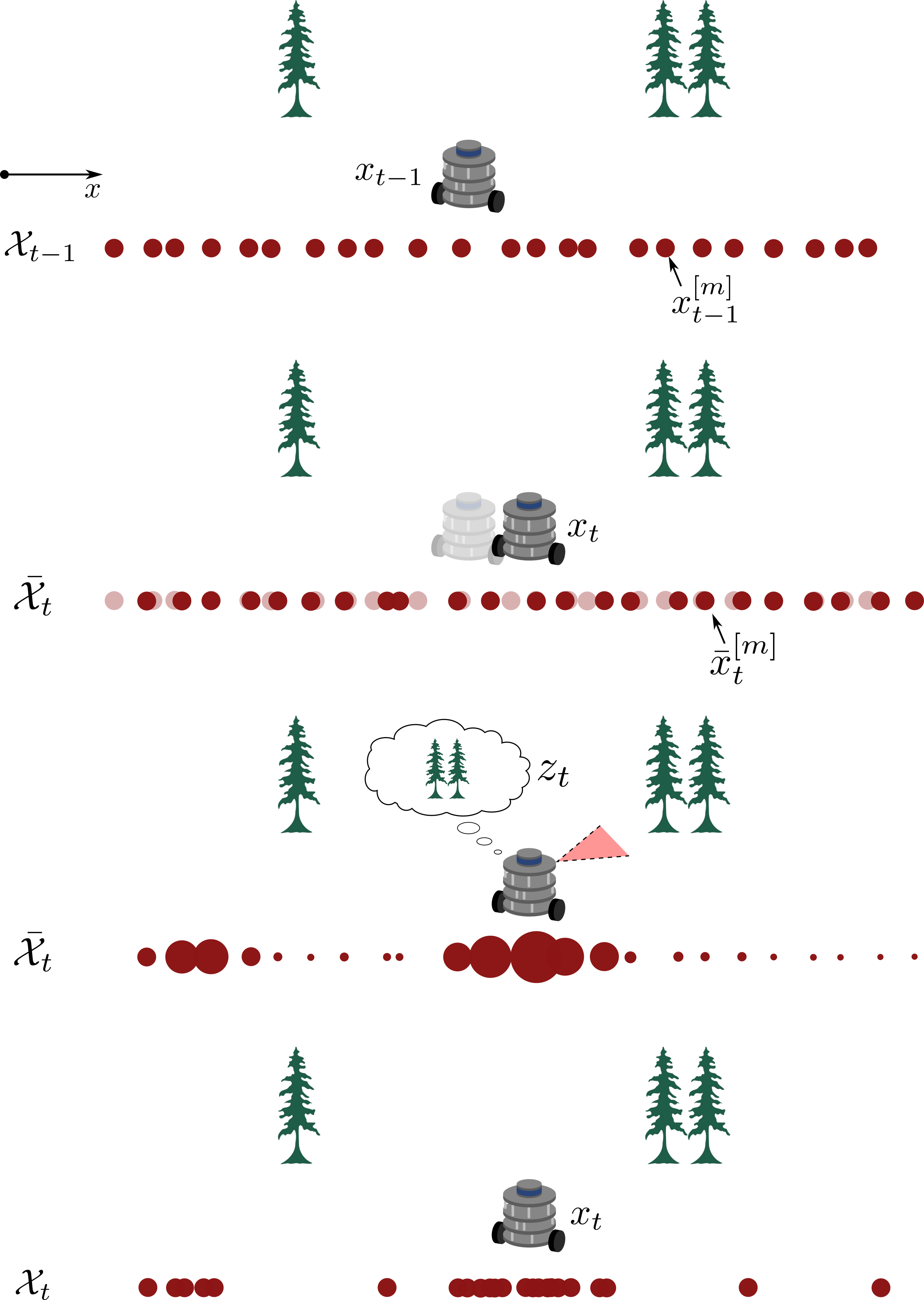
The particle filter’s measurement update step then consists of resampling (with replacement) a new set of $K$ particles from $\bar{\mathcal{P}}_{t}$ , according to the normalized weights $w_{t}^{[k]}$ . Particles with large weights are likely to be selected many times, while particles with negligible weights may disappear. The resampled set $\mathcal{P}_{t}$ approximates the updated belief $\text{bel}(\bm{x}_{t})$ .

We summarize the algorithm in Algorithm 5 and illustrate a few iterations of the particle filter for a simple robot localization problem in Figure 12.1.

The resampling step is important for more than just incorporating the measurement. Without resampling, repeated multiplication of weights would gradually concentrate probability on a tiny subset of particles, while most particles would have negligible weight and effectively be wasted. This phenomenon is known as particle degeneracy. Resampling combats degeneracy by repeatedly discarding low-weight particles and replicating high-weight particles, keeping the effective sample size roughly constant.

This effect has a nice interpretation in evolutionary terms: particles that explain the data well “survive and reproduce”, while those that do not are gradually removed. From a computational perspective, resampling focuses particles in high-probability regions of the state space and reduces the number of particles required for a given level of accuracy.

Refer to caption — Figure 12.1: A particle filter used for robot localization. We first update the initial set of particles according to the transition model, and then weight them according to the observation. Finally, we generate a new set of particles through weighted resampling.

12.5 Summary

In this chapter, we examined practical approximations to the Bayes filter for continuous and high-dimensional state estimation problems in robotics. We began by motivating the need for tractable filtering methods and introduced two broad families of approximate filters, parametric and non-parametric, each with its own strengths and weaknesses.

Parametric filters, such as the Kalman filter and its nonlinear extensions, the EKF and the UKF, represent the belief as a Gaussian distribution, enabling efficient recursive updates of mean and covariance. We discussed how these filters exploit linear or locally linear models to achieve computational efficiency, along with their limitations in representing multimodal or highly nonlinear beliefs.

We then introduced non-parametric filters, including the histogram and particle filters, which relax parametric assumptions and directly approximate the belief distribution through discretization or sampling. These methods trade additional computation for representational flexibility, making them effective in situations involving global uncertainty, nonlinear dynamics, or non-Gaussian noise.

Table 12.1: Parametric vs. Non-parametric Filters (at a glance)

	Parametric (KF / EKF / UKF)	Non-parametric (Histogram / Particle)
Belief	Single Gaussian (mean, covariance)	Grid masses or weighted samples
Nonlinearity	EKF (linearize), UKF (sigma points)	Native; no Jacobians needed
Multimodality	Poor (unimodal)	Natural (multi-peak)
Dimensionality	Scales well with state dim	Histogram: suffers; Particle: scalable with $K$
Computation	Cheap per step	Histogram: grows with bins; Particle: $O(K)$
When it shines	Smooth models, near-Gaussian noise, good observability	Ambiguity, strong nonlinearities, non-Gaussian noise, global localization
Pitfalls	Linearization bias (EKF), covariance inconsistency	Degeneracy without resampling; sample impoverishment

Table 12.1 summarizes the main characteristics of these approaches and highlights their complementary strengths. In practice, robotic systems often combine elements of both families in order to balance accuracy, robustness, and computational efficiency.

High-level decision guide.

It is useful to relate common robotics scenarios to appropriate filter architectures. Kalman-style filters are well suited for local tracking problems with smooth motion and reliable sensors, whereas histogram or particle filters are better suited for global localization, ambiguous data association, or highly nonlinear environments.

1.

If the robot’s dynamics or sensing models are mildly nonlinear and beliefs stay near unimodal $\Rightarrow$ EKF.
2.

If the Jacobians of the dynamics or sensor models are hard to compute or their nonlinearities are significant $\Rightarrow$ UKF (or square-root UKF).
3.

If there is global or multimodal uncertainty, or severe non-Gaussian noise $\Rightarrow$ Particle filter.
4.

If the state is low-dimensional and a map or grid is available $\Rightarrow$ Histogram filter.

To learn more.

For a comprehensive and accessible treatment of probabilistic state estimation and filtering methods, readers are encouraged to consult the classic text by Thrun et al. (2005)²2. Thrun, S., Burgard, W., Fox, D. Probabilistic Robotics. MIT Press, 2005.. Detailed derivations and discussions of Kalman filtering theory can also be found in Maybeck (1982)³3. Maybeck, Peter S. Stochastic models, estimation, and control. Academic press, 1982., while Julier and Uhlmann (1997)⁴4. Julier, Simon J, Uhlmann, Jeffrey K. “New extension of the Kalman filter to nonlinear systems.” In Signal processing, sensor fusion, and target recognition VI, 182–193, 1997. provide the seminal introduction to the Unscented Kalman Filter. For further reading on non-parametric filters and their applications to robot localization, see Dellaert et al. (1999)⁵5. Dellaert, Frank, Fox, Dieter, Burgard, Wolfram, Thrun, Sebastian. “Monte carlo localization for mobile robots.” In Proceedings 1999 IEEE international conference on robotics and automation (Cat. No. 99CH36288C), 1322–1328, 1999.. A modern perspective that unifies filtering, smoothing, and mapping under a probabilistic framework is presented in SLAM Handbook. From Localization and Mapping to Spatial Intelligence⁶6. SLAM Handbook. From Localization and Mapping to Spatial Intelligence. Cambridge University Press, 2026., which connects the foundations of state estimation to contemporary SLAM and spatial-AI systems.

12.6 Exercises

The starter code for the exercises provided below is available online through GitHub. To get started, download the code by running in a terminal window:

⬇

git clone https://github.com/StanfordASL/pora-exercises.git

We denote Problems requiring hand-written solutions and coding in Python with and , respectively.

Problem 1: Kalman Filter for Landmark Localization

In this exercise, you will implement a Kalman Filter to localize a set of fixed landmarks given knowledge about a robot’s motion. Specifically, consider an environment where there are four landmarks, and we define the state of landmark positions as the vector:

\begin{split}\bm{x}_{t}^{m}=\begin{bmatrix}x_{t}^{m_{1}}&y_{t}^{m_{1}}&x_{t}^{% m_{2}}&y_{t}^{m_{2}}&x_{t}^{m_{3}}&y_{t}^{m_{3}}&x_{t}^{m_{4}}&y_{t}^{m_{4}}% \end{bmatrix}^{\top},\end{split}

which we assume we can directly measure (i.e. $\bm{z}_{t}=\bm{x}_{t}$ ) with a noisy sensor.

In the file ch12/exercises/kalman_filter.ipynb, perform the following tasks:

1.

Define the state transition matrix $A$ from Equation 12.3 and observation matrix $C$ from Equation 12.4 for the Kalman filter algorithm. The matrix $A$ should correspond to the motion of the landmarks, which we assume are stationary, and $C$ should represent the direct measurement of the landmark positions.
2.

Implement the Kalman filter predict and update steps to compute the means and covariances at each time step.
3.

Run the provided code to see the results.

Practice · 2 notebooks

Ekf Ukf Range Bearing Open in Colab Source
Kalman Filter Open in Colab Source