The filtering algorithms developed in Chapter 11 and Chapter 12 provide general tools for estimating the state of a dynamical system from noisy measurements. In mobile robotics, one of the most important instances of this general problem is localization: estimating a robot’s pose with respect to a map of the environment.
In this chapter, we specialize the Bayesian filtering framework to the robot localization problem. We begin in Section 13.1 with a taxonomy that organizes different localization scenarios—pose tracking versus global localization, static versus dynamic environments, active versus passive sensing, and single-robot versus multi-robot settings. This taxonomy provides a mental model for the kinds of problems that arise in practice.
In Section 13.2, we then express localization formally as a Bayesian filtering problem in which the state is the robot pose and the map is an additional, known variable that influences both motion and measurements. This leads to map-aware state transition and measurement models, which we discuss in Section 13.3.
Building on this formulation, in Section 13.4 we introduce Markov localization, a general Bayes filter for estimating a robot’s pose that explicitly incorporates a map. Markov localization is conceptually clean but rarely implemented directly; instead, it serves as a reference from which more specialized algorithms are derived.
We then present two specializations of Markov localization. In Section 13.5, we develop an EKF localization algorithm for feature-based maps that are well suited to pose tracking with moderate uncertainty. Finally, in Section 13.6 we introduce Monte Carlo Localization (MCL), a particle filter–based method that can handle global localization and strongly multimodal beliefs. Along the way, we discuss data association and practical considerations that arise in map-based localization.
13.1 A Taxonomy of Robot Localization Problems
| Axis | Representative cases | Typical algorithmic implications |
|---|---|---|
| Initial pose | Pose tracking (local), global localization, kidnapped robot | Tracking often amenable to unimodal Gaussian filters; global and kidnapped scenarios typically require non-parametric, multimodal beliefs (e.g., particle filters). |
| Environment | Static, slowly varying, strongly dynamic | Static maps simplify modeling; dynamic elements motivate robust measurement models and possibly explicit dynamic object tracking. |
| Action selection | Passive, active (information-seeking) | Passive use treats controls as given; active localization couples the filter with planning methods that trade off task progress and information gain. |
| Number of robots | Single robot, multi-robot (cooperative) | Multi-robot settings introduce shared maps and inter-robot observations, leading to coupled estimation problems and opportunities for improved robustness. |
Robot localization problems can differ substantially depending on how much is known about the initial pose, how the environment evolves, how actions are chosen, and how many robots are involved. Before turning to specific algorithms, it is helpful to organize these variations using a taxonomy.
We will use the term pose to refer to the robot’s position and orientation in a global coordinate frame. For a planar mobile robot, the pose is typically at time , where is the planar position and is the heading angle.
Pose tracking and global pose localization.
One of the first distinctions among robot localization problems concerns what we assume we know about the initial pose:
-
•
Pose tracking (local localization). In pose tracking problems, the initial pose is known with reasonably small uncertainty. For example, a robot may be placed at a known charging station or docking location, with a prior belief concentrated in a small neighborhood. The goal is to maintain an accurate estimate of pose over time as the robot moves and senses, despite process and measurement noise.
-
•
Global localization. In global localization, the robot has very little prior information about its initial pose. For instance, it may know only that it is somewhere within a building, but not which floor, corridor, or room. The belief over poses must therefore represent multiple plausible hypotheses, often spread over a large region of the map.
-
•
Kidnapped robot problem. A challenge related to global localization arises when a robot that has been successfully tracking its pose is suddenly transported to a different, unknown location without its sensors or localization algorithm being aware of the event. This kidnapped robot problem requires the localization method to recover from a grossly incorrect belief and reinitialize globally.
Pose tracking problems are often amenable to unimodal Gaussian approximations, such as EKF-based methods, whereas global localization and kidnapped robot scenarios typically require non-parametric methods capable of representing multiple hypotheses, such as histogram or particle filters.
Static and dynamic environment localization.
A second axis in the taxonomy of robot localization concerns how the environment changes over time:
-
•
Static environments. In the simplest case, the environment map is fixed and does not change. Walls and landmarks remain in place, and any moving objects (such as people) are ignored or treated as noise. Many foundational localization algorithms are developed under this assumption.
-
•
Dynamic environments. In more realistic settings, parts of the environment change over time. Examples include doors that open and close, furniture that moves, or other agents that occupy the same space. In these cases, the map may be time varying or may explicitly model dynamic objects.
In this chapter, we primarily consider localization with respect to a static map, while allowing for noisy measurements that may occasionally be corrupted by dynamic elements. Handling fully dynamic maps is closely related to SLAM and tracking, and will be revisited in Chapter 14.
Active and passive localization.
Localization algorithms also differ in how they interact with the environment:
-
•
Passive localization. In passive localization, the algorithm treats the sequence of controls as given; it does not attempt to choose actions to improve localization performance. Many navigation systems fall into this category when localization is treated as a background process.
-
•
Active localization. In active localization, the robot chooses its actions with the explicit goal of reducing uncertainty about its pose. For example, the robot may move to viewpoints that disambiguate map symmetries or collect measurements that are expected to be highly informative.
The algorithms developed in this chapter apply in both settings. When used in an active framework, they provide the state and uncertainty estimates needed for planning information-seeking actions.
Single and multi-robot localization.
Finally, localization problems can involve one or multiple robots:
-
•
Single-robot localization. A single robot must estimate its pose using on-board sensors and possibly an external reference, such as GPS, relative to a map that we assume is given.
-
•
Multi-robot localization. In multi-robot settings, several robots localize simultaneously, often sharing information. Robots may observe each other, exchange measurements, or maintain a shared map. This introduces additional structure and opportunities for cooperation, but also coupling between the individual localization problems.
Throughout this chapter, we focus on single-robot localization in a known, largely static map. The methods we develop form the basis for more advanced multi-robot and SLAM systems.
13.2 Robot Localization via Bayesian Filtering
In previous chapters, we introduced several well-known variations of the Bayes filter, including the parametric EKF and the non-parametric particle filter in Chapter 12. These algorithms propagate a belief distribution over a state using a probabilistic Markov state transition model and a probabilistic measurement model. Recall that for a general state-space model, the belief at time is defined as:
| (13.1) |
where are all measurements up to time and are the applied controls.
In map-based localization, the state represents the robot pose, and we assume that a map of the environment is given. The map encodes information about the environment that constrains both how the robot can move and what it can measure. Our goal is to compute the posterior over robot poses conditioned on the map:
To incorporate the map into the filtering framework, we modify both the state transition model and the measurement model. Specifically, in Section 13.3, we introduce a map-aware state transition model that captures the fact that some poses are inconsistent with the environment. Then, in Section 13.3.1, we introduce a map-aware measurement model that reflects how local sensor readings depend on nearby structures in the map. The combination of these two models leads directly to the localization algorithms we introduce in Section 13.5 and Section 13.6.
Map representation.
Before modifying the probabilistic models, it is useful to briefly review how we represent maps in this chapter. We assume that the environment can be described by a collection of spatial entities—either discrete landmarks or volumetric cells—with associated properties. Formally, we denote the map as:
where each element describes a portion of the environment.
Depending on the application, may represent the occupancy state of a grid cell (occupied/free/unknown), the position of a point landmark, in a global frame, or more complex attributes such as semantic labels or reflectivity. We will use the generic term “map element” for , and refer informally to these as “objects” or “cells” when helpful.

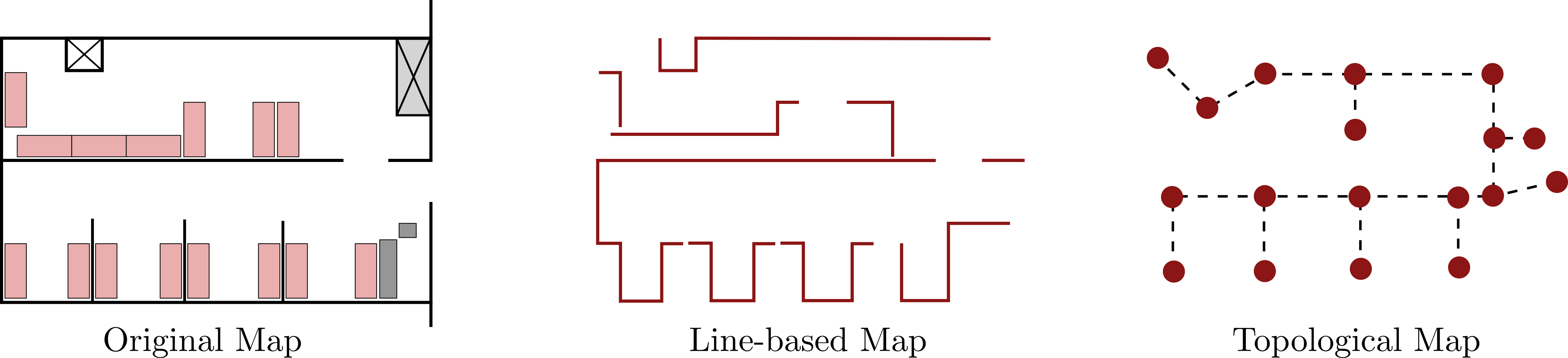
Two important map families arise frequently in mobile robotics:
-
•
Feature-based maps, where each is a compact feature, such as a point landmark or line segment, with precisely defined geometry. Figure 13.2 shows two examples of feature-based maps, one represented by lines and another by a graph of nodes and edges.††margin: Graph-based maps are generally referred to as topological maps.
-
•
Cell-based (occupancy grid) maps, where the environment is discretized into a grid of cells, each with an associated occupancy probability. This is closely related to the grid-based motion planning representations discussed in the referenced section. Figure 13.1 shows examples where the environment is represented by a set of volumetric cells.
Cell-based maps trade off resolution and computational cost: smaller cells provide finer spatial detail but increase memory usage and computation time, while larger cells reduce cost but blur detail and can misrepresent narrow passages. We refer back to the grid-based planning discussion in the referenced section for a deeper treatment of these trade-offs. In this chapter, we treat the choice of map representation as given, and focus on how the map enters the filtering equations.
13.3 Map-Aware State Transition Model
The map influences how the robot can move. For example, a mobile robot cannot pass through walls or leave the known workspace. A purely kinematic transition model does not capture these constraints: it might assign nonzero probability to states that lie inside obstacles or outside the mapped area.
To incorporate the map, we consider the map-aware transition model . Directly modeling this distribution for arbitrary maps is difficult, so we adopt an approximation that reuses the original transition model and a separate, map-induced prior. Specifically, we define as the probability of a pose given only the map. This term characterizes how consistent a pose is with the environment. For example, for a pose inside a wall or outside the mapped region.
Using Bayes’ rule, we can approximate the map-aware transition model as:
| (13.2) |
where is a normalization constant that ensures the left-hand side integrates to one. Equation 13.2 can be derived step-by-step by starting from Bayes’ rule:
Since does not depend on , we can absorb it into a constant :
Next, we assume that the influence of the past on the map is captured entirely through the current pose :
Intuitively, once we know the current pose, the specific path taken to get there does not provide additional information about the static map.111This approximation becomes more accurate as the time step between and shrinks, so that the robot moves only a short distance between successive poses. With this assumption:
Applying Bayes’ rule again to gives:
Substituting into the previous expression and absorbing constant factors that do not depend on into a new normalization constant yields:
which is Equation (Equation 13.2).
In this approximation, is the probability of a state given only the map and captures the geometric consistency of that state with respect to the environment††margin: For example, for a state that lies inside a wall or outside the known map. . The factor encodes the motion model, and acts as a map-based correction that suppresses physically implausible states.
From a computational perspective, Equation (Equation 13.2) is attractive because it allows us to reuse existing implementations of the motion model and incorporate the map through a relatively inexpensive correction:
-
•
We first generate a kinematic prediction of the new pose using , which depends only on the robot model and control.
-
•
We then reweight or prune these predictions using , which often reduces to simple operations such as checking whether the pose lies in free space (for occupancy grids) or near a corridor (for semantic maps).
Thus, the map-aware transition model modifies the likelihood of proposed poses without requiring a complete redesign of the underlying motion model.
13.3.1 Map-Aware Measurement Model
The map also strongly influences sensor measurements. For instance, the range returned by a lidar beam depends on where that beam first intersects an obstacle in the map, and the bearing to a visual landmark depends on the landmark’s position in the global frame. To reflect this dependence, we introduce a map-aware measurement model:
In many systems, a measurement vector consists of individual components, such as individual range beams or landmark observations. A common simplifying assumption is that the individual components of the measurement vector are conditionally independent given the state and map. Under this assumption, we can factor the measurement model as:
| (13.3) |
The conditional independence assumption is not exact. For example, nearby range beams may be correlated if they hit the same object. However, this assumption greatly simplifies inference and works well in many practical settings. It allows us to process multiple sensor readings either in a batch or sequentially, using the same underlying model for each component.
13.4 Markov Localization
The first map-based localization algorithm we introduce is Markov localization. Markov localization applies the Bayes filter from Chapter 11 to the map-aware models introduced above. The belief over robot pose at time is:
and the map is treated as known and fixed.
Using the map-aware transition and measurement models and , the Bayes filter recursion becomes:
where denotes the predicted belief and is a normalization constant chosen so that . We summarize this recursion in Algorithm 1.
Conceptually, Markov localization has the same structure as the Bayes filter from Chapter 11: a prediction step that propagates the belief through the motion model, followed by a correction step that incorporates the latest measurement. The only difference is that both the prediction and correction now depend explicitly on the map .
In its most general form, however, Markov localization is not directly computationally tractable. The integral over all possible poses and the need to maintain an arbitrary belief function are prohibitive in high-dimensional or continuous state spaces. As in Chapter 12, the key to practicality is to choose a representation for the belief that is expressive enough for the problem at hand, yet structured enough to admit efficient computation.
In Section 13.5, we adopt a unimodal Gaussian belief and derive an EKF-based localization algorithm, which is well suited for pose tracking with moderate uncertainty. In Section 13.6, we adopt a particle-based representation and derive Monte Carlo Localization, capable of handling global localization and multimodal beliefs.
13.5 EKF Localization
We now develop an EKF-based realization of Markov localization. The EKF localization algorithm assumes that the belief over the robot’s pose can be approximated by a single Gaussian:
and applies the EKF prediction and update equations from Chapter 12 using map-aware models. This Gaussian structure significantly improves computational efficiency relative to the full Markov localization algorithm, at the cost of not being able to represent multiple well-separated pose hypotheses.222As in Chapter 12, this unimodality assumption is well suited to pose tracking but generally insufficient for global localization.
We assume the same nonlinear state transition model as in the referenced section:
where is zero-mean Gaussian process noise. The corresponding state transition Jacobian is:
| (13.4) |
where is the mean of the previous belief .
The main difference between the general EKF and EKF localization is the presence of a feature-based map and a measurement model that relates robot poses to observed landmarks. We assume we have a map of point landmarks:
where each landmark is given by its two-dimensional location in the global coordinate frame. At time the robot obtains a set of landmark measurements:
where each is associated (implicitly or explicitly) with one landmark.
Given a pose and the index of the corresponding landmark, the measurement model is:
where models zero-mean Gaussian sensor noise, and encodes the expected range, bearing, or other features to landmark . For each measurement, the Jacobian of the measurement model with respect to the state is:
| (13.5) |
where is the predicted mean from the EKF prediction step, and is the index of the map feature associated with measurement .
A new challenge in feature-based localization is data association. Given a set of measurements , which landmark does each measurement correspond to? We denote the correspondence for measurement at time by , where means that measurement corresponds to landmark , and indicates that measurement does not correspond to any known landmark††margin: For example, due to a spurious detection. .
We first consider the simpler case where we assume the correspondences are known.
13.5.1 EKF Localization with Known Correspondences
Assume for the moment that the correspondences are known. The EKF localization algorithm then resembles the standard EKF from Chapter 12, with two key modifications:
-
1.
The measurement model relates the pose to map features via .
-
2.
Multiple landmark measurements are processed at each time step.
Given the pose and the map , and given known correspondences , the joint likelihood of the measurement set can be written as:
Using the conditional independence assumption from Equation 13.3—now applied at the level of individual landmark measurements—we have:
Each factor is a Gaussian distribution whose mean is given by and whose covariance is .
Because the prior over is Gaussian and each measurement likelihood term is Gaussian, the posterior remains Gaussian. Moreover, under the conditional independence assumption, we can apply the standard EKF measurement update sequentially for each and obtain the same result as if we had processed all measurements in a single stacked update. This is a consequence of the fact that, for Gaussian models, multiplication of likelihood terms can be carried out in any order.
Algorithm 2 summarizes the EKF localization recursion in the known-correspondence case. This algorithm provides a useful baseline: if we knew which measurement came from which landmark, EKF localization would be a straightforward specialization of the standard EKF. The main additional difficulty in practice is that the correspondences are typically unknown and must be estimated jointly with the robot state.
13.5.2 EKF Localization with Unknown Correspondences
In realistic scenarios, the correspondences are not given and must be inferred from the data. One common approach is to estimate the correspondences using a maximum likelihood (MLE) criterion. At each time step, we choose to maximize the likelihood of the current measurements:
In words, we select the assignment of measurements to landmarks that makes the observed data most probable, given the map and the past history.
To make this optimization tractable, we first marginalize over the unknown pose :
where we used the Markov assumption to simplify , and defined the predicted belief:
The term is the measurement model with known correspondences. Using the conditional independence assumption from Equation 13.3, we can factor it as:
Substituting into the integral, we obtain:
Although the measurements are conditionally independent given , they become coupled after marginalizing over . A common approximation is therefore to select correspondences independently by scoring each measurement-landmark pairing under the predicted belief:
Under the Gaussian assumptions on the belief and measurement model, the integral above is a Gaussian distribution with mean and covariance:
where:
Maximizing the likelihood is therefore equivalent to choosing to maximize the Gaussian density , or equivalently to minimize the associated Mahalanobis distance:
| (13.6) |
where:
| (13.7) |
is the Mahalanobis distance between the actual measurement and its prediction under landmark .
In practice, additional validation gates are often imposed: if the minimum distance exceeds a threshold, the measurement is treated as unmatched (assigned to the “no landmark” index ) and excluded from the EKF update. Once the correspondences have been determined, they are treated as known in Algorithm 3, yielding the full EKF localization algorithm with unknown correspondences.
Example 13.5.1 (Differential drive robot with range and bearing measurements).
Consider a differential drive robot with state and a sensor that measures the range and bearing to landmarks in the robot’s local coordinate frame. We assume that at each time step the robot collects multiple measurements corresponding to different features:
where each measurement contains the range and bearing .
Assuming the correspondences are known, the measurement model for the range and bearing of landmark is:
| (13.8) |
The measurement Jacobian corresponding to a measurement from landmark is therefore:
| (13.9) |
It is also common to assume a diagonal covariance for the measurement noise:
where is the standard deviation of the range measurement noise and is the standard deviation of the bearing measurement noise. This reflects the assumption that range and bearing errors are uncorrelated.
13.6 Monte Carlo Localization (MCL)
The second practical realization of Markov localization we consider is Monte Carlo localization (MCL). This algorithm leverages the non-parametric particle filter framework from Chapter 12 and is particularly well suited to global pose localization and the kidnapped robot problem.††margin: We can also use MCL to solve the kidnapped robot problem by injecting new randomly sampled particles at each step so that the filter remains sensitive to unexpected measurements.
Like the particle filter, MCL represents the belief distribution by a set of particles:
where each particle represents a hypothesis about the true state . Regions of the state space with more particles correspond to higher belief.
At each step of the algorithm, we:
-
1.
propagate particles forward using the map-aware state transition model, and
-
2.
weight and resample the particles using the map-aware measurement model.
This is summarized in Algorithm 4, which is nearly identical to the particle filter algorithm in the referenced algorithm, the only difference being that the map now appears in the probabilistic state transition and measurement models.
In global localization, MCL typically starts from a broad prior, such as having particles spread over the entire map. As the robot moves and gathers measurements, inconsistent hypotheses are down-weighted and vanish during resampling, while particles near the true pose accumulate. This makes MCL a powerful tool for environments with strong ambiguities, repeated structures, or very uncertain initial conditions.
13.7 Summary
In this chapter, we examined the fundamental concepts and algorithms underlying robot localization—the process of estimating a robot’s pose relative to a known map of the environment. We began with a taxonomy of localization problems, distinguishing between pose tracking and global localization, static and dynamic environments, active and passive strategies, and single-robot versus multi-robot settings. This taxonomy provides a conceptual checklist for matching real-world scenarios to appropriate algorithmic tools.
Building on the Bayesian estimation framework introduced earlier, we extended the state transition and measurement models to explicitly incorporate map information. This led to the Markov localization algorithm, a general Bayesian filter that serves as a conceptual foundation for map-aware localization.
We then explored two important realizations of this framework: EKF localization, which represents the belief as a unimodal Gaussian and is effective for pose tracking with moderate uncertainty; and MCL, which uses a particle-based, non-parametric representation suitable for multi-hypothesis and global localization problems. We discussed data association—the challenge of determining correspondences between sensor measurements and known map features—and techniques such as maximum-likelihood matching and validation gates to improve robustness.
Together, these methods form the core of modern localization systems, enabling robots to estimate their position and orientation using noisy sensors, partial maps, and uncertain environments. In later chapters, these ideas will reappear in more complex settings such as simultaneous localization and mapping (SLAM), where the robot must estimate both its pose and the map at the same time.
To learn more.
For a detailed and foundational treatment of probabilistic localization, Thrun et al. (2005)11. Thrun, S., Burgard, W., Fox, D. Probabilistic Robotics. MIT Press, 2005. remains the canonical reference. The original formulation of the Monte Carlo Localization algorithm is presented by Dellaert et al. (1999)22. Dellaert, Frank, Fox, Dieter, Burgard, Wolfram, Thrun, Sebastian. “Monte carlo localization for mobile robots.” In Proceedings 1999 IEEE international conference on robotics and automation (Cat. No. 99CH36288C), 1322–1328, 1999., while Leonard and Durrant-Whyte (1991)33. Leonard, John J, Durrant-Whyte, Hugh F. “Simultaneous map building and localization for an autonomous mobile robot..” In IROS, 1442–1447, 1991. provide an early and influential treatment of EKF-based localization with geometric landmarks. Readers interested in recent advances and the connection between localization and SLAM may refer to Cadena et al. (2017)44. Cadena, Cesar, Carlone, Luca, Carrillo, Henry, Latif, Yasir, Scaramuzza, Davide, Neira, José, Reid, Ian, Leonard, John J. “Past, present, and future of simultaneous localization and mapping: Toward the robust-perception age.” IEEE Transactions on robotics 32(6), 1309–1332, 2017. and the comprehensive modern text by SLAM Handbook. From Localization and Mapping to Spatial Intelligence55. SLAM Handbook. From Localization and Mapping to Spatial Intelligence. Cambridge University Press, 2026., which unify localization and mapping under a common probabilistic and optimization-based framework.
13.8 Exercises
The starter code for the exercises provided below is available online through GitHub. To get started, download the code by running in a terminal window:
We denote Problems requiring hand-written solutions and coding in Python with ![[Uncaptioned image]](/book-assets/robot-localization/figs__write.png) and
and ![[Uncaptioned image]](/book-assets/robot-localization/figs__code.png) , respectively.
, respectively.
Problem 1: Extended Kalman Filter Localization
In this problem, you will implement an extended Kalman filter (EKF) for robot localization in an environment where the robot can collect relative position measurements to a set of four landmarks. We will consider a robot with a discrete-time dynamics model defined by:
and the goal is to estimate the unknown robot pose, . The noise vector is a random variable with a zero mean Gaussian distribution , where . In this problem, we assume the global ground truth positions of the four landmarks are known. The landmarks are stationary objects in the environment, and their combined state vector is:
As the robot navigates through its environment, it receives noisy measurements of the positions of four landmarks in the environment relative to the robot’s current pose. The measurement for landmark is the relative position with the measurement model:
where the measurements have an associated measurement noise with , where . The full measurement vector of all landmarks is:
In the file ch13/exercises/ekf_localization.ipynb, complete the following:
-
1.
Implement the functions robot_dynamics and robot_measurement to match the dynamics and measurement models described above.
-
2.
Implement the function dynamics_jacobian to compute the dynamics Jacobian .
-
3.
Implement the function measurement_jacobian to compute the measurement model Jacobian for the model that computes the full measurement vector .
-
4.
Implement the function ekf_localization_update to implement the EKF localization update described in Algorithm 2. Note that you won’t need to explicitly have a for loop in this function for each measurement since we have defined the update to be vectorized for all measurements at once.
-
5.
Run the provided code to see how the algorithm performs for the simulated robot.
Problem 2: Particle Filter Localization
In this problem, we consider the same problem setup defined in Problem 1, where we are localizing a robot given relative position measurements to a set of four known landmarks. In the file ch13/exercises/particle_filter_localization.ipynb, complete the following:
-
1.
Implement the functions robot_dynamics and robot_measurement to match the dynamics and measurement models described above. Note: you can reuse your solution from the previous problem.
-
2.
Implement the particle filter algorithm update function particle_filter_update as described in Algorithm 4.
-
3.
Run the provided code to see how the algorithm performs for the simulated robot.
Practice · 2 notebooks
- Ekf Localization Open in Colab Source
- Particle Filter Localization Open in Colab Source