Introduction to Localization and Filtering · Principles of Robot Autonomy

We have already discussed the robot motion planning problem and surveyed common algorithms for it, ranging from optimal control to sampling-based methods. All of these approaches implicitly assume access to the robot’s current state, for example for initializing trajectory optimization methods or for closing the loop in feedback control. In practice, however, this state cannot be read directly; it must be estimated from noisy, partial sensor data.

Robot perception, as introduced in previous chapters, tackles the challenge of extracting semantic and geometric information from raw sensor streams. These methods are indispensable for local, instantaneous awareness. For instance, detecting nearby obstacles with a laser scanner or identifying objects in view with a camera. Yet this information is inherently local and relative to the robot’s current position. It suffices for collision avoidance, but not for the global reasoning required by full planning and control schemes.

This gap is addressed by robot localization and mapping, one of the core components of the “think” stage in the classical “see-think-act” cycle. The goal of robot localization and mapping is to synthesize local sensor data into a coherent global estimate of the robot’s state and map the surrounding environment. In this chapter, we focus on localization, which is the ability to infer the robot’s current state with respect to a global frame or map ⁶6. Thrun, S., Burgard, W., Fox, D. Probabilistic Robotics. MIT Press, 2005.
Siegwart, R., Nourbakhsh, I. R., Scaramuzza, D. Introduction to Autonomous Mobile Robots. MIT Press, 2011.. For instance, before a robot can navigate to a target room on the floor plan shown in Figure 11.1, it must first establish where in the building it is located.

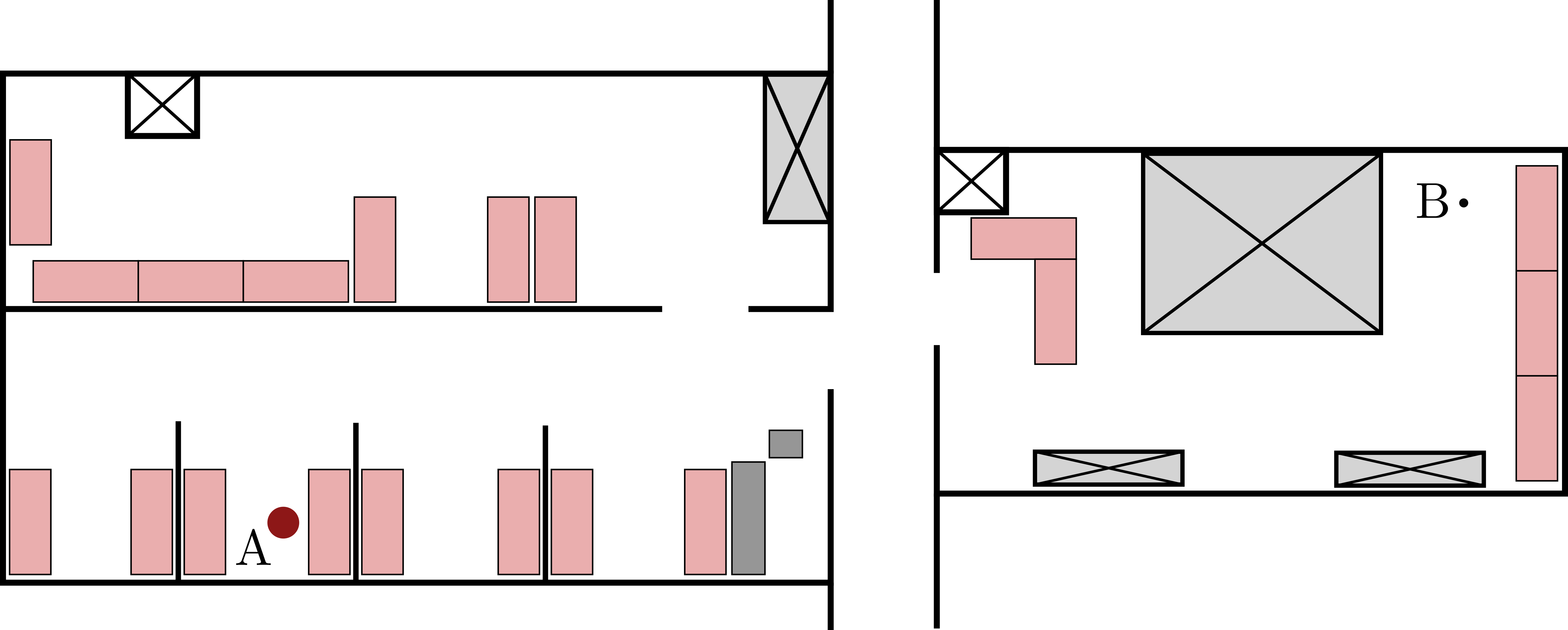
Refer to caption — Figure 11.1: Localization is crucial for autonomy: to move from A to B, the robot must know which room it occupies, and that the only path to B runs through the hallway. Inferring such global information from local range measurements requires specialized algorithms.

A central challenge in localization is uncertainty. Sensor data is noisy, incomplete, and sometimes ambiguous. To handle this, localization is cast in a probabilistic framework: instead of maintaining a single guess of the robot’s state, we maintain a belief distribution over possible states. This representation allows us to extract both point estimates and measures of uncertainty. Uncertainty quantification is vital for downstream tasks. For example, a planner may avoid high-risk trajectories under localization uncertainty, or even select actions that deliberately reduce uncertainty through information gathering.

The rest of this chapter is organized as follows. In Section 11.1, we review key concepts in probability theory, including random variables, probability distributions, conditional probabilities, and Bayes’ rule. In Section 11.2, we introduce Markov models as a probabilistic representation of robot motion and sensing. Finally, in Section 11.3, we derive the Bayes filter, a recursive algorithm for maintaining and updating a belief distribution as controls are applied and new measurements arrive.

11.1 Preliminary Concepts in Probability

Tools from probability theory provide us with a way to systematically reason about uncertainty in robotics. Specifically, these tools provide the language to model noisy sensor measurements, uncertain robot states, and stochastic environments. In this section, we review several key building blocks that form the foundation for probabilistic filtering algorithms such as the Bayes filter, namely random variables, probability distributions, conditional probabilities, and Bayes’ rule.

11.1.1 Random Variables

We can model uncertain quantities in robotics, such as sensor measurements, robot states, or environmental properties, as random variables. Depending on the domain of possible values, random variables are classified as discrete or continuous.

Definition 11.1 (Discrete random variable).

A discrete random variable $X$ takes values from a countable set. The probability that $X$ takes on a specific value $x$ is denoted by $p(X=x)$ , or more compactly $p(x)$ . The function $p(x)$ is called the probability mass function (PMF), and it must satisfy:

\sum_{x}p(x)=1,

where the sum is over all possible values of $X$ .

Definition 11.2 (Continuous random variable).

A continuous random variable $X$ takes values in an uncountable set, typically a subset of $\mathbb{R}^{n}$ . Its distribution is characterized by a probability density function (PDF) $p(x)$ , which satisfies:

\int_{-\infty}^{\infty}p(x)\,dx=1.

Unlike the discrete case, the probability that a continuous random variable takes on any exact value is zero:

P(X=x)=0.

Intuitively, this is because a single point has zero width and probability mass only accumulates over intervals. Consequently, probabilities are defined over regions rather than individual values. For example, the probability that $X$ lies in the interval $[a,b]$ is:

P(a\leq X\leq b)=\int_{a}^{b}p(x)\,dx.

Example 11.1.1 (Discrete vs. continuous random variables).

A coin flip is a discrete random variable, $X\in\{\text{heads},\text{tails}\}$ , with a probability mass function:

p(\text{heads})=\tfrac{1}{2},\qquad p(\text{tails})=\tfrac{1}{2}.

In robotics, we typically model the robot’s pose as a continuous random variable. For example, a planar robot pose $\bm{x}\in SE(2)$ ^†^†margin: $SE(2)$ is the special Euclidean group in two dimensions. It represents planar rigid-body transformations and consists of a position $(x,y)$ and an orientation $\theta$ . For robots operating in three-dimensional space, the pose lies in $SE(3)$ , which represents 3D position and orientation. can take infinitely many values because both its position and orientation vary continuously.

Probability distributions.

The probability mass function for discrete random variables and probability density function for continuous random variables are often collectively referred to as probability distributions. There are many ways to parameterize a probability distribution. For discrete variables, the distribution can be specified explicitly by assigning a probability to each possible value. For continuous variables, the distribution is often described by a parametric function defined by a small number of parameters. Choosing an appropriate representation is important in robotics, since it determines both how uncertainty is modeled and how efficiently algorithms can reason about it.

11.1.2 Joint Distributions, Independence, and Conditioning

Many robotics problems involve more than one uncertain quantity at a time. For example, a robot might simultaneously reason about its pose, the position of an obstacle, and a sensor reading. In such cases, it is useful to describe the probabilities of multiple random variables together using a joint distribution.

Definition 11.3 (Joint distribution).

The joint distribution of two random variables $X$ and $Y$ specifies the probability that both take on specific values simultaneously. It is denoted by $p(X=x,\,Y=y)$ , or more compactly $p(x,y)$ .

Independence.

Random variables can be related to each other in important ways. For example, the random variables $X=$ “today is cloudy” and $Y=$ “today it is raining” are correlated: if there are no clouds, it is unlikely to rain. In contrast, two random variables are probabilistically independent if the value of one does not provide any information about the other.

Definition 11.4 (Probabilistic independence).

Two random variables $X$ and $Y$ are probabilistically independent if and only if:

p(x,y)=p(x)\,p(y).

(11.1)

Example 11.1.2 (Independent sensor measurements).

Suppose a robot uses a proximity sensor and a temperature sensor, modeled by random variables $X$ and $Y$ . Let $X\in\{\text{close},\text{medium},\text{far}\}$ and $Y\in\{\text{low},\text{med},\text{high}\}$ , with $p(X=\text{close})=1/3$ and $p(Y=\text{med})=1/5$ . If the two sensors are independent, the joint probability of observing “close” and “med” is:

p(X=\text{close},\,Y=\text{med})=\tfrac{1}{3}\cdot\tfrac{1}{5}=\tfrac{1}{15}.

Conditional probability.

Another key concept is the probability of one random variable given that another has already been observed.

Definition 11.5 (Conditional probability).

The conditional probability of a random variable $X$ taking value $x$ , given that $Y$ took value $y$ , is:

p(x\mid y)\coloneqq\frac{p(x,y)}{p(y)}.

(11.2)

Conditional probabilities allow us to update beliefs when new information becomes available. If $X$ and $Y$ are independent, then $p(x\mid y)=p(x)$ , meaning that knowing $Y$ provides no additional information about $X$ .

Example 11.1.3 (Sensor conditional probabilities).

Building on Example 11.1.2, consider an obstacle detection variable $Z\in\{\text{detected},\text{not detected}\}$ . Assume that the detection probability depends on the proximity sensor value:

\begin{split}p(Z=\text{detected}\mid X=\text{close})&=\tfrac{5}{6},\\ p(Z=\text{detected}\mid X=\text{medium})&=\tfrac{1}{3},\\ p(Z=\text{detected}\mid X=\text{far})&=\tfrac{1}{5}.\end{split}

If $p(X=\text{close})=\frac{1}{3}$ , then the probability that the robot both detects an obstacle and registers “close” is:

\begin{split}p(Z=\text{detected},\,X=\text{close})&=p(Z=\text{detected}\mid X=% \text{close})\,p(X=\text{close})\\ &=\tfrac{5}{18}.\end{split}

Conditional independence.

Finally, independence can also hold given the outcome of another variable. This concept is known as conditional independence and plays a central role in probabilistic modeling.

Definition 11.6 (Conditional independence).

Two random variables $X$ and $Y$ are said to be conditionally independent given a third variable $Z$ if:

p(x,y\mid z)=p(x\mid z)\,p(y\mid z),

(11.3)

for all values of $x$ , $y$ , and $z$ . Equivalently:

p(x\mid y,z)=p(x\mid z).

(11.4)

We denote conditional independence as:

X\perp Y\mid Z.

Intuitively, conditional independence means that once the value of $Z$ is known, learning the value of $Y$ provides no additional information about $X$ . However, if $Z$ is not known, the variables $X$ and $Y$ may still appear correlated. In other words, the variable $Z$ explains the dependence between $X$ and $Y$ .

Example 11.1.4 (Conditional independence in robotics).

A mobile robot equipped with two wheel encoders produces measurements of traveled distance: one from the left wheel ( $X$ ) and one from the right wheel ( $Y$ ). At first glance, these two measurements may seem correlated, since the robot’s motion affects both. However, if we condition on the underlying hidden variable $Z$ = “true distance traveled,” the two encoder readings are independent:

p(x,y\mid z)=p(x\mid z)\,p(y\mid z).

That is, once the actual distance traveled is known, the left and right encoder readings do not provide additional information about each other. This is a typical use of conditional independence in probabilistic sensor models.

11.1.3 Law of Total Probability

The law of total probability links marginal, joint, and conditional probabilities. It provides a systematic way to compute the probability of one random variable by accounting for all possible outcomes of another.

Definition 11.7 (Law of total probability).

For discrete random variables $X$ and $Y$ :

p(x)=\sum_{y}p(x,y)=\sum_{y}p(x\mid y)\,p(y).

For continuous random variables:

p(x)=\int p(x,y)\,dy=\int p(x\mid y)\,p(y)\,dy.

Intuitively, the law of total probability states that to find the probability of $X$ taking value $x$ , we can sum (or integrate) over all possible values of $Y$ , weighting the conditional probability of $X$ given each value of $Y$ by the probability of that value of $Y$ itself. This process is known as marginalization, and $p(x)$ is called the marginal probability of $X$ .

Example 11.1.5 (Robot localization via marginalization).

Suppose a robot’s position $X$ depends on which hallway $Y$ it is currently in. We can compute the probability of being at a particular location $x$ by considering every possible hallway $y$ :

p(x)=\sum_{y}p(x\mid y)\,p(y).

In practice, this means we marginalize over the possible hallways, combining both the likelihood of being in each hallway and the probability of observing $x$ given that hallway.

11.1.4 Bayes’ Rule

The joint probability, $p(x,y)$ , between two random variables, $X$ and $Y$ , is related to the conditional probabilities, $p(x\mid y)$ and $p(y\mid x)$ , from the definition of a conditional probability in Equation 11.2. Since we can express the joint probability using either conditional probability, we have:

p(x,y)=p(x\mid y)p(y)=p(y\mid x)p(x).

This relationship is commonly referred to as Bayes’ rule^†^†margin: Sometimes also referred to as Bayes’ theorem. .

Definition 11.8 (Bayes’ rule).

For discrete random variables, $X$ and $Y$ , Bayes’ rule states that:

p(x\mid y)=\frac{p(y\mid x)p(x)}{p(y)}.

(11.5)

Bayes’ rule is useful because it provides a relationship between the “inverse” conditional probabilities, $p(x\mid y)$ and $p(y\mid x)$ . This is particularly important for probabilistic inference problems where we need to infer the value of one random variable from another. For example, suppose we have a good initial guess of the probability distribution^†^†margin: When we have an estimate of the probability distribution $p(x)$ before any new information is used to update it, we will refer to it as the prior probability. , $p(x)$ , for a random variable, $X$ . Given new information about the outcome of a second random variable, $Y$ , that is related to $X$ , we can use Bayes’ rule to update our belief about the probability distribution of $X$ by computing $p(x\mid y)$ ^†^†margin: This new distribution, which we obtained by updating the prior distribution $p(x)$ with the new information about $Y$ , is commonly referred to as the posterior probability. . Bayes’ rule also extends to cases with additional random variables. For example, with three random variables, $X$ , $Y$ , and $Z$ , Bayes’ rule is:

p(x\mid y,z)=\frac{p(y\mid x,z)p(x\mid z)}{p(y\mid z)}.

Example 11.1.6 (Bayes’ rule).

Consider a scenario where a robot is trying to figure out if it is in room A or room B inside of a building. The robot has an initial guess that the probability it is in room A is $p(A)=\frac{3}{4}$ , and the robot has a camera that can be used to improve the estimate. Suppose that a single image, $I$ , is captured and the features extracted from the image are compared to the known room features which gives the conditional probabilities:

p(I\mid A)=\frac{3}{4},\quad p(I\mid B)=\frac{1}{2}.

We can use Bayes’ rule to compute the posterior probability:

p(A\mid I)=\frac{p(I\mid A)p(A)}{p(I)},

where we use the law of total probability to compute:

p(I)=p(I,A)+p(I,B)=p(I\mid A)p(A)+p(I\mid B)p(B),

and using $p(B)=1-p(A)$ .

11.1.5 Expectation, Variance, and Covariance

Probability distributions describe uncertainty in full detail by assigning probabilities to every possible outcome of a random variable. In practice, however, we often summarize a distribution using more compact statistics. Some of the most common statistics used to summarize a distribution include the expected value, variance, and covariance.

Expectation.

The expectation of a random variable is a measure of the central tendency of its distribution.

Definition 11.9 (Expectation).

The expectation^†^†margin: Also referred to as the mean or the first moment of a distribution. of a random variable $X$ is denoted by $\mathbb{E}\left[X\right]$ . For discrete random variables:

\mathbb{E}\left[X\right]=\sum_{x}x\,p(x),

where the sum is over all outcomes of $X$ . For continuous random variables:

\mathbb{E}\left[X\right]=\int x\,p(x)\,dx.

The expected value can be interpreted as the average outcome obtained if the random variable were sampled repeatedly an infinite number of times.

The expectation has several useful properties. One particularly important property is linearity, which states that the expectation of a linear transformation of a random variable is equal to the linear transformation of the expectation of the random variable. Formally, for any random variable $X$ and constants $a,b\in\mathbb{R}$ , we have:

\mathbb{E}\left[aX+b\right]=a\mathbb{E}\left[X\right]+b.

This property holds regardless of the distribution of $X$ .

For vector-valued random variables $\bm{X}=[X_{1},\ldots,X_{n}]^{\top}$ , the expectation is defined component-wise:

\mathbb{E}\left[\bm{X}\right]=\begin{bmatrix}\mathbb{E}\left[X_{1}\right]\\ \vdots\\ \mathbb{E}\left[X_{n}\right]\end{bmatrix}.

Variance.

While the expected value describes the center of a distribution, it does not capture how uncertain the variable is. This uncertainty is measured by the variance.

Definition 11.10 (Variance).

The variance of a random variable $X$ is defined as:

\text{Var}(X)=\mathbb{E}\left[(X-\mathbb{E}\left[X\right])^{2}\right].

The variance measures the average squared deviation of the variable from its mean. A large variance indicates that the variable can take values far from the mean, while a small variance indicates that the variable is tightly concentrated around the mean. The square root of the variance is called the standard deviation, often denoted by $\sigma$ .

Covariance.

When dealing with multiple random variables, it is often important to understand how their uncertainties are related. This relationship is captured by the covariance.

Definition 11.11 (Covariance).

The covariance between two random variables $X$ and $Y$ is denoted $\text{cov}(X,Y)$ and defined as:

\begin{split}\text{cov}(X,Y)&=\mathbb{E}\left[(X-\mathbb{E}\left[X\right])(Y-% \mathbb{E}\left[Y\right])^{\top}\right]\\ &=\mathbb{E}\left[XY^{\top}\right]-\mathbb{E}\left[X\right]\,\mathbb{E}\left[Y% \right]^{\top}.\end{split}

Intuitively, the covariance describes how two random variables vary together. If the covariance is positive, the variables tend to increase or decrease together. If it is negative, one variable tends to increase when the other decreases. If the covariance is zero, the variables are uncorrelated.

Example 11.1.7 (Robot motion uncertainty).

Suppose $X$ represents the forward displacement of a robot and $Y$ represents its lateral displacement during a single motion step. If wheel slip increases as the robot moves farther forward, then larger values of $X$ tend to be associated with larger sideways deviations, producing a positive covariance between $X$ and $Y$ .

Conversely, if the robot’s mechanical design or control system tends to stabilize lateral motion during forward travel, the covariance between $X$ and $Y$ may be negative. If forward and lateral displacements arise from unrelated sources, the covariance will be close to zero.

11.2 Markov Models

In Chapter 1, we modeled robot motion using kinematics and dynamics, obtaining a set of first-order differential equations (see the referenced equation) that deterministically describe how the state $\bm{x}$ evolves in time given the current state and control input $\bm{u}$ . In this section, we generalize this view to a probabilistic setting by introducing Markov models, which describe how the state evolves under uncertainty. Markov models are fundamental to robotics, appearing in localization, mapping, planning, and decision-making under uncertainty problems.

State, controls, and measurements.

As in Chapter 1, the state $\bm{x}\in\mathbb{R}^{n}$ collects all variables relevant to the task at hand. In motion planning and control, this typically includes the robot’s physical state (pose, velocity, etc.), while in localization or higher-level planning it may also include environment variables such as landmark positions or object features. We work in discrete time, writing $\bm{x}_{t}$ for the state at time $t$ . We also use the shorthand $\bm{x}_{t_{1}:t_{n}}\coloneqq\bm{x}_{t_{1}},\bm{x}_{t_{2}},\ldots,\bm{x}_{t_{n}}$ for sequences of states, with analogous notation for control inputs $\bm{u}_{t_{1}:t_{n}}$ and measurements $\bm{z}_{t_{1}:t_{n}}$ .^†^†margin: Measurements can come from any of the sensors introduced earlier, such as cameras, lidar, or inertial units.

Unlike deterministic dynamics, Markov models specify probability distributions over possible states and observations. In full generality, the state evolution is modeled as:

p(\bm{x}_{t}\mid\bm{x}_{0:t-1},\bm{z}_{1:t-1},\bm{u}_{1:t}),

(11.6)

which captures the distribution of the current state $\bm{x}_{t}$ conditioned on the entire history of past states, controls, and measurements. Following the convention used throughout this chapter, the robot first executes the control $\bm{u}_{t}$ , then receives the measurement $\bm{z}_{t}$ based on the resulting state $\bm{x}_{t}$ . The corresponding probabilistic measurement model is:

p(\bm{z}_{t}\mid\bm{x}_{0:t},\bm{z}_{1:t-1},\bm{u}_{1:t}).

(11.7)

The Markov property.

In many applications, we define the state $\bm{x}_{t}$ to be complete, meaning it contains all the information necessary to predict future states. Formally, this assumption implies that past states and measurements provide no additional predictive power beyond $\bm{x}_{t-1}$ and $\bm{u}_{t}$ . This is known as the Markov property, under which the models simplify to:

p(\bm{x}_{t}\mid\bm{x}_{t-1},\bm{u}_{t}),

(11.8)

for the state transition, and:

p(\bm{z}_{t}\mid\bm{x}_{t}),

(11.9)

for the measurement model.

Markov models in robotics.

A Markov model thus consists of a state transition distribution (Equation 11.8) and a measurement distribution (Equation 11.9). Intuitively, the transition model captures process uncertainty (e.g., wheel slip when applying a control), while the measurement model captures sensor noise (e.g., rangefinder variability). Together, these components form the foundation of probabilistic state estimation (Figure 11.2).

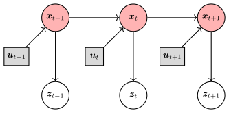
diagram — Figure 11.2: Graphical representation of a Markov model. At each time step, the control $\bm{u}_{t}$ influences the new state $\bm{x}_{t}$ , and the resulting state generates a measurement $\bm{z}_{t}$ .

The probabilistic model described above belongs to a broader family of models that assume the system state evolves according to the Markov property. Several closely related formulations exist, depending on whether control inputs and observability are considered.

In robotics, the state of the system is typically not directly observable. Instead, sensors provide indirect and noisy measurements that depend on the underlying state. Models with this structure are often referred to as partially observable Markov models.

If control inputs are not present, the model reduces to a hidden Markov model (HMM). In this case, the state evolves according to a Markov process, and observations provide partial information about that state. The term “hidden” reflects the fact that the true state $\bm{x}_{t}$ cannot be observed directly and must instead be inferred from the sequence of measurements.

11.3 Bayes Filter

Robot localization is a classic instance of a filtering problem^†^†margin: Localization is one instance of the more general filtering problem referred to as state estimation. where our goal is to compute a probability distribution over the current state $\bm{x}_{t}$ given the history of control inputs $\bm{u}_{1:t}$ , and measurements $\bm{z}_{1:t}$ . One of the canonical approaches to this filtering problem is known as the Bayes filter or recursive Bayesian estimation. The Bayes filter leverages a Markov model to recursively update a belief distribution, which is a probability distribution over $\bm{x}_{t}$ . Mathematically, we denote the belief distribution as $\text{bel}(\bm{x}_{t})$ and define it as:

\text{bel}(\bm{x}_{t})\coloneqq p(\bm{x}_{t}\mid\bm{z}_{1:t},\bm{u}_{1:t}).

(11.10)

In other words, the belief $\text{bel}(\bm{x}_{t})$ is a posterior probability distribution over the state conditioned on the available history information. We also define a distribution called the prediction distribution as:

\overline{\text{bel}}(\bm{x}_{t})\coloneqq p(\bm{x}_{t}\mid\bm{z}_{1:t-1},\bm{% u}_{1:t}),

(11.11)

which does not include the most recent measurement $\bm{z}_{t}$ . We call the process of using the new measurement $\bm{z}_{t}$ to compute the belief $\text{bel}(\bm{x}_{t})$ from the predicted belief $\overline{\text{bel}}(\bm{x}_{t})$ a correction or measurement update. The Bayes filter consists of a prediction step for computing $\overline{\text{bel}}(\bm{x}_{t})$ from the prior belief followed by a correction step for computing $\text{bel}(\bm{x}_{t})$ given the new measurement $\bm{z}_{t}$ .

11.3.1 Algorithm

The recursive structure of the Bayes filter is summarized in Algorithm 1. At each time step, the filter maintains a belief distribution belief $\text{bel}(\bm{x}_{t})$ over the system state. The inputs to the filter are the previous belief^†^†margin: In practice, we initialize the prior distribution $\text{bel}(\bm{x}_{0})$ using either a best guess of the initial state or a uniform distribution when no prior information is available. , the current control input $\bm{u}_{t}$ , and the latest sensor measurement $\bm{z}_{t}$ .

The algorithm proceeds in two stages. First, a prediction step computes the distribution $\overline{\text{bel}}(\bm{x}_{t})$ over possible states after applying the control input. This step propagates uncertainty forward using the state transition model from Equation 11.8. Second, a correction step incorporates the new measurement using the measurement model from Equation 11.9, adjusting the predicted belief to better match the observed data.

Intuitively, the prediction step estimates where the robot might be after executing the control, while the correction step refines this estimate using information from the sensors.

Data:

\text{bel}(\bm{x}_{t-1}),\bm{u}_{t},\bm{z}_{t}

Result:

\text{bel}(\bm{x}_{t})

foreach $\bm{x}_{t}$ do

// Prediction (motion update)

\overline{\text{bel}}(\bm{x}_{t})=\int p(\bm{x}_{t}\mid\bm{x}_{t-1},\bm{u}_{t}%)\,\text{bel}(\bm{x}_{t-1})\,d\bm{x}_{t-1}

// Correction (measurement update)

\text{bel}(\bm{x}_{t})=\eta\,p(\bm{z}_{t}\mid\bm{x}_{t})\,\overline{\text{bel}%}(\bm{x}_{t})

return

\text{bel}(\bm{x}_{t})

Algorithm 1 Bayes Filter

In Algorithm 1, $\eta$ is a normalization constant ensuring $\text{bel}(\bm{x}_{t})$ integrates (or sums) to one.^†^†margin: In practice, $\eta=1/p(\bm{z}_{t}\mid\bm{z}_{1:t-1},\bm{u}_{1:t})$ , which follows directly from Bayes’ rule. Conceptually, the Bayes filter performs a repeated predict–correct cycle, where the motion model spreads the belief forward to account for process uncertainty, while the measurement model reshapes the belief according to how consistent each state is with the observed sensor measurement.

11.3.2 Derivation

We now derive the Bayes filter recursion from the definition of the belief distribution introduced in Section 11.3. Applying Bayes’ rule to Equation 11.10 yields:

\begin{split}\text{bel}(\bm{x}_{t})&=p(\bm{x}_{t}\mid\bm{z}_{1:t},\bm{u}_{1:t}% )\\ &=\eta\,p(\bm{z}_{t}\mid\bm{x}_{t},\bm{z}_{1:t-1},\bm{u}_{1:t})\,p(\bm{x}_{t}% \mid\bm{z}_{1:t-1},\bm{u}_{1:t}),\end{split}

(11.12)

where $\eta$ is a normalization constant:

\eta=\frac{1}{p(\bm{z}_{t}\mid\bm{z}_{1:t-1},\bm{u}_{1:t})}.

Measurement update.

Using the conditional independence assumptions of the Markov model (Figure 11.2), the current measurement depends only on the current state. Therefore:

p(\bm{z}_{t}\mid\bm{x}_{t},\bm{z}_{1:t-1},\bm{u}_{1:t})=p(\bm{z}_{t}\mid\bm{x}% _{t}).

Substituting this simplification into Equation 11.12 gives:

\text{bel}(\bm{x}_{t})=\eta\,p(\bm{z}_{t}\mid\bm{x}_{t})\,p(\bm{x}_{t}\mid\bm{% z}_{1:t-1},\bm{u}_{1:t}).

Recall the definition of the prediction belief from Equation 11.11:

\overline{\text{bel}}(\bm{x}_{t})\coloneqq p(\bm{x}_{t}\mid\bm{z}_{1:t-1},\bm{% u}_{1:t}),

we obtain:

\text{bel}(\bm{x}_{t})=\eta\,p(\bm{z}_{t}\mid\bm{x}_{t})\,\overline{\text{bel}% }(\bm{x}_{t}),

which corresponds to the measurement update step of the Bayes filter.

Prediction update.

Next we derive an expression for the prediction belief $\overline{\text{bel}}(\bm{x}_{t})$ . Starting from its definition in Equation 11.11, we apply the law of total probability to marginalize over the previous state $\bm{x}_{t-1}$ :

\begin{split}\overline{\text{bel}}(\bm{x}_{t})&=\int p(\bm{x}_{t},\bm{x}_{t-1}% \mid\bm{z}_{1:t-1},\bm{u}_{1:t})d\bm{x}_{t-1}\\ &=\int p(\bm{x}_{t}\mid\bm{x}_{t-1},\bm{z}_{1:t-1},\bm{u}_{1:t})p(\bm{x}_{t-1}% \mid\bm{z}_{1:t-1},\bm{u}_{1:t})d\bm{x}_{t-1}.\end{split}

Using the Markov assumption again, the next state depends only on the previous state and the current control input:

p(\bm{x}_{t}\mid\bm{x}_{t-1},\bm{z}_{1:t-1},\bm{u}_{1:t})=p(\bm{x}_{t}\mid\bm{% x}_{t-1},\bm{u}_{t}).

Furthermore, the control input $\bm{u}_{t}$ does not influence the previous state $\bm{x}_{t-1}$ , so:

p(\bm{x}_{t-1}\mid\bm{z}_{1:t-1},\bm{u}_{1:t})=p(\bm{x}_{t-1}\mid\bm{z}_{1:t-1% },\bm{u}_{1:t-1}).

Recognizing that, by definition:

\text{bel}(\bm{x}_{t-1})=p(\bm{x}_{t-1}\mid\bm{z}_{1:t-1},\bm{u}_{1:t-1}),

we obtain the prediction step:

\overline{\text{bel}}(\bm{x}_{t})=\int p(\bm{x}_{t}\mid\bm{x}_{t-1},\bm{u}_{t}% )\,\text{bel}(\bm{x}_{t-1})\,d\bm{x}_{t-1}.

11.3.3 Discrete Bayes Filter

When the state space is finite, the belief distribution can be represented as a probability mass function over a discrete set of states $\{x_{k}\}$ . In this case, the belief at time $t$ is described by a collection of probabilities $\{p_{k,t}\}$ , where $p_{k,t}$ denotes the probability that the system is in state $x_{k}$ at time $t$ . The Bayes filter recursion can then be written in discrete form by replacing the integrals in Algorithm 1 with summations over the possible states. The resulting algorithm, shown in Algorithm 2, follows the same two-step procedure as the continuous Bayes filter, with a prediction step using the transition model, followed by a correction step using the measurement model.

Data:

\{p_{k,t-1}\},\bm{u}_{t},\bm{z}_{t}

Result:

\{p_{k,t}\}

foreach $k$ do

\overline{p}_{k,t}=\sum_{i}p(\bm{x}_{t}\mid\bm{x}_{i},\bm{u}_{t})\,p_{i,t-1}

p_{k,t}=\eta\,p(\bm{z}_{t}\mid\bm{x}_{k})\,\overline{p}_{k,t}

return

\{p_{k,t}\}

Algorithm 2 Discrete Bayes Filter

Here $\overline{p}_{k,t}$ denotes the predicted probability of state $x_{k}$ before incorporating the measurement, and $\eta$ is a normalization constant ensuring that the probabilities sum to one.

11.3.4 Practical Considerations

The Bayes filter provides a general and principled framework for probabilistic state estimation. However, applying it directly is often computationally challenging in realistic robotics problems.

In continuous state spaces, the prediction step requires evaluating integrals over the entire state space. Computing these integrals exactly is often intractable, resulting in the need for approximations or numerical methods to estimate the belief distribution. In discrete state spaces, the recursion can be computed exactly, but the required summations scale with the number of possible states. As the dimensionality of the state increases, the number of discrete states grows rapidly, making exact inference computationally expensive.

Despite these challenges, the Bayes filter serves as the conceptual foundation for many practical state estimation algorithms. Widely used filters such as the Kalman filter, extended Kalman filter (EKF), unscented Kalman filter (UKF), and particle filter can all be viewed as specific implementations of the Bayes filter that exploit additional assumptions or approximations to make the computation tractable.

Example 11.3.1 (Robot in a hallway).

Consider a robot moving along a straight hallway represented by a one-dimensional line. The hidden state $\bm{x}_{t}$ is the robot’s position along this line. At each time step $t$ the robot receives a control input $\bm{u}_{t}$ representing a commanded forward displacement and a measurement $\bm{z}_{t}$ representing the noisy distance to the nearest door in front of the robot, obtained from a range sensor.

Prediction.

Suppose the robot starts at position $\bm{x}_{t-1}=2$ m with a belief concentrated around that location and issues a command $\bm{u}_{t}=+0.5$ m forward. Due to wheel slip and actuator noise, the true displacement may vary, which we model as:

\Delta x\sim\mathcal{N}(u_{t},\,0.1^{2}).

The prediction step therefore spreads the belief forward, producing belief $\overline{\text{bel}}(\bm{x}_{t})$ centered at $2.5$ m but with larger variance than the previous belief.

Correction.

At the same step, the robot’s range sensor reports $\bm{z}_{t}=2.4$ m to the next door. The sensor is noisy and modeled by:

p(\bm{z}_{t}\mid\bm{x}_{t})=\mathcal{N}(\bm{z}_{t};\text{true distance}(\bm{x}% _{t}),\,0.05^{2}).

If the predicted belief assigns significant probability to states near $\bm{x}_{t}\approx 2.5$ m and the hallway map indicates that the next door lies roughly $2.4$ m ahead from that position, the measurement is consistent with the prediction. The correction step therefore increases the probability of these states and sharpens the belief distribution around them. States that would predict very different measurements are downweighted.

Recursive operation.

Over time, the filter alternates prediction and correction. The prediction step tends to broaden the belief because motion introduces uncertainty, while the correction step can concentrate the belief when informative measurements are received. In hallways with repeating structures, several positions may initially produce similar sensor readings, causing the belief to remain multimodal. As the robot gathers additional observations, the Bayes filter resolves this ambiguity and the belief collapses around the robot’s true location.

In the repository github.com/StanfordASL/pora-exercises, the notebook ch11/discrete_bayes.ipynb provides a concrete implementation of the discrete Bayes filter for this hallway example. Running the notebook illustrates how the belief distribution evolves over time as the robot moves and collects measurements.

11.4 Summary

In this chapter, we introduced the probabilistic foundations underlying robot localization and state estimation. We began by motivating why localization is essential for autonomy: robots must infer their pose from noisy and partial sensor data rather than directly observing it. To reason systematically about this uncertainty, we reviewed key concepts in probability theory, including random variables, probability distributions, conditional independence, and Bayes’ rule. These concepts provide the mathematical framework for representing and updating uncertainty in robotic systems.

Building on these foundations, we introduced Markov models as probabilistic representations of robot motion and sensing. These models define how the robot’s state evolves over time and how measurements relate to that state, forming the basis for probabilistic inference in dynamic systems. Finally, we derived the Bayes filter, a recursive algorithm for estimating a belief distribution over the robot’s state as it moves and collects new measurements. The Bayes filter provides the conceptual foundation for many practical estimation algorithms. Widely used methods such as the Kalman filter, extended Kalman filter, unscented Kalman filter, and particle filter can all be understood as specific implementations of this general framework. In the following chapters, we build on these ideas to develop practical algorithms for localization, mapping, and simultaneous localization and mapping.

To learn more.

For a comprehensive introduction to probabilistic robotics, including localization and filtering, readers are referred to the seminal text by Thrun et al. (2005)¹1. Thrun, S., Burgard, W., Fox, D. Probabilistic Robotics. MIT Press, 2005., which provides an intuitive and rigorous treatment of the Bayes filter and its extensions. Additional foundational perspectives on probabilistic reasoning and estimation in robotics can be found in Siegwart et al. (2011)²2. Siegwart, R., Nourbakhsh, I. R., Scaramuzza, D. Introduction to Autonomous Mobile Robots. MIT Press, 2011. and Maybeck (1982)³3. Maybeck, Peter S. Stochastic models, estimation, and control. Academic press, 1982.. For readers interested in a more theoretical background in stochastic systems and control, Gelb et al. (1974)⁴4. Gelb, Arthur et al. Applied optimal estimation. MIT press, 1974. offers a classical reference on estimation theory. Finally, SLAM Handbook. From Localization and Mapping to Spatial Intelligence⁵5. SLAM Handbook. From Localization and Mapping to Spatial Intelligence. Cambridge University Press, 2026. presents a modern, unified treatment of localization, filtering, and mapping under a common probabilistic framework.

11.5 Exercises

The starter code for the exercises provided below is available online through GitHub. To get started, download the code by running in a terminal window:

⬇

git clone https://github.com/StanfordASL/pora-exercises.git

We denote Problems requiring hand-written solutions and coding in Python with and , respectively.

Problem 1: Airport Security

Suppose that travelers passing through an airport carry prohibited items $1\%$ of the time. Each passenger passes through a simple detector that has a true positive detection rate of $92\%$ and false positive detection rate of $8\%$ . Passengers that trigger the detector alarm are sent to a more accurate secondary screening that has a true positive detection rate of $98\%$ and a false positive detection rate of $10\%$ .

1.

Given that a randomly selected passenger was flagged by the second screening, what is the probability a passenger was carrying a prohibited item?
2.

How does the probability change in this case if all passengers were to get the more accurate secondary screening and the first simple detector was not used?

Problem 2: Cookie Machine

You operate a cookie-making machine that when activated will produce a random number of cookies in the range $[1,\dots,N]$ , with each quantity equally likely with probability $\frac{1}{N}$ . Each cookie costs $\$1$ to produce.

1.

Each of your customers will pay a fixed price to activate the machine. What is the minimum fixed price you should charge each customer to ensure that you don’t lose money in the long run? In other words, what is the expected cost of each customer activation?

Suppose the machine manufacturer produces machines with $N=6$ and $N=10$ , and unfortunately they don’t know which one they sent you, but the chance you received either machine is equally likely. However, they did record that in a test run of your machine it produced $5$ cookies.

2.

What is the probability that you received a machine configured with $N=6$ ?
3.

What is the expected number of cookies that will be produced the first time you operate the machine?

Practice · 1 notebooks

Discrete Bayes Open in Colab Source