Camera Models and Calibration

The two main kinds of sensors used in digital cameras today are charge-coupled devices (CCD) and complementary metal-oxide-semiconductor (CMOS) sensors. A CCD chip is an array of light-sensitive picture elements called pixels, and can contain between 20,000 and several million pixels total. We can think of each pixel as a light-sensitive discharging capacitor that is $5$ to $25\mu \text{m}$ in size. While complementary metal oxide semiconductor (CMOS) chips also consist of an array of pixels, they are quite different from CCD chips. In particular, along the side of each pixel are several transistors specific to that pixel. CCD sensors have typically outperformed CMOS for quality-sensitive applications such as digital single-lens-reflex cameras, while CMOS sensors are better for low-power applications. However, today, CMOS sensors are standard in most digital cameras.

Rays of light reflected by an object tend to be scattered in many directions and may consist of different wavelengths. Averaged over time, the emitted wavelengths and directions for a specific object can be precisely described using object-specific probability distribution functions. In particular, the light reflection properties of a given object are the result of how light is reflected, scattered, or absorbed based on the object’s surface properties and the wavelength of the light. For example, an object might look blue because blue wavelengths of light are primarily scattered off the surface while other wavelengths are absorbed.

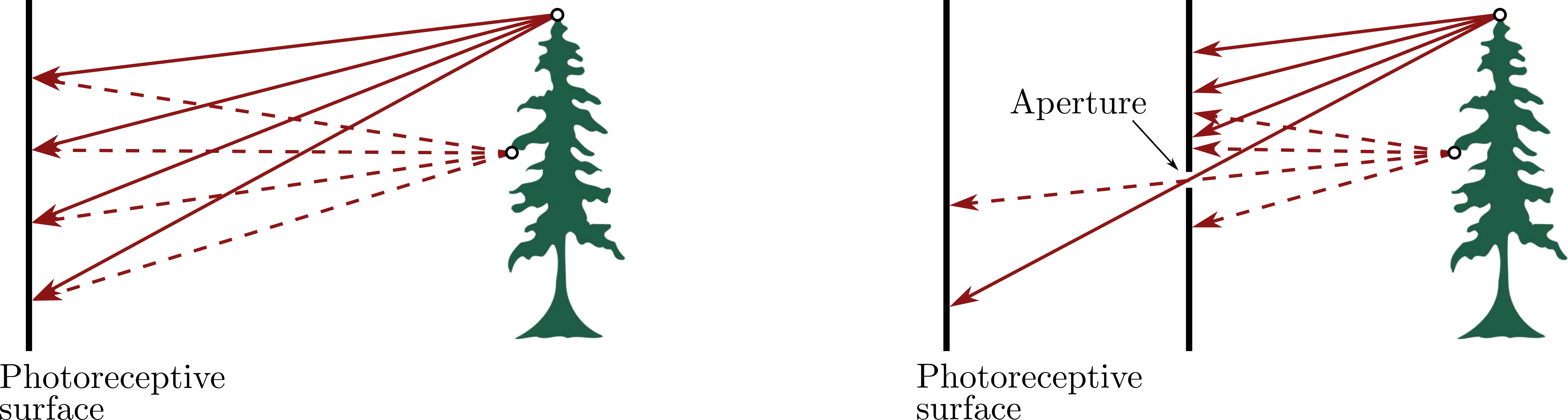
Cameras capture images by sensing reflected light rays on a photoreceptive surface such as a CCD or a CMOS sensor. Since light reflecting off an object is generally scattered in many directions, exposing a planar photoreceptive surface to these reflected rays would result in many rays being captured at each pixel, which would lead to blurry images. A solution to this issue is to add a barrier in front of the photoreceptive surface that only lets some of the rays pass through an aperture, as we show in Figure 6.1. The earliest approach to filtering light rays in this way was to have a small hole in the barrier surface. We refer to cameras with this type of filter as pinhole cameras.

A pinhole camera has no lens but rather a single small aperture. Light from the scene passes through this pinhole aperture and projects an inverted image onto the image plane, as we show in Figure 6.2. While modern cameras do not operate in this way, we can use the principles of the pinhole camera to derive useful mathematical models.

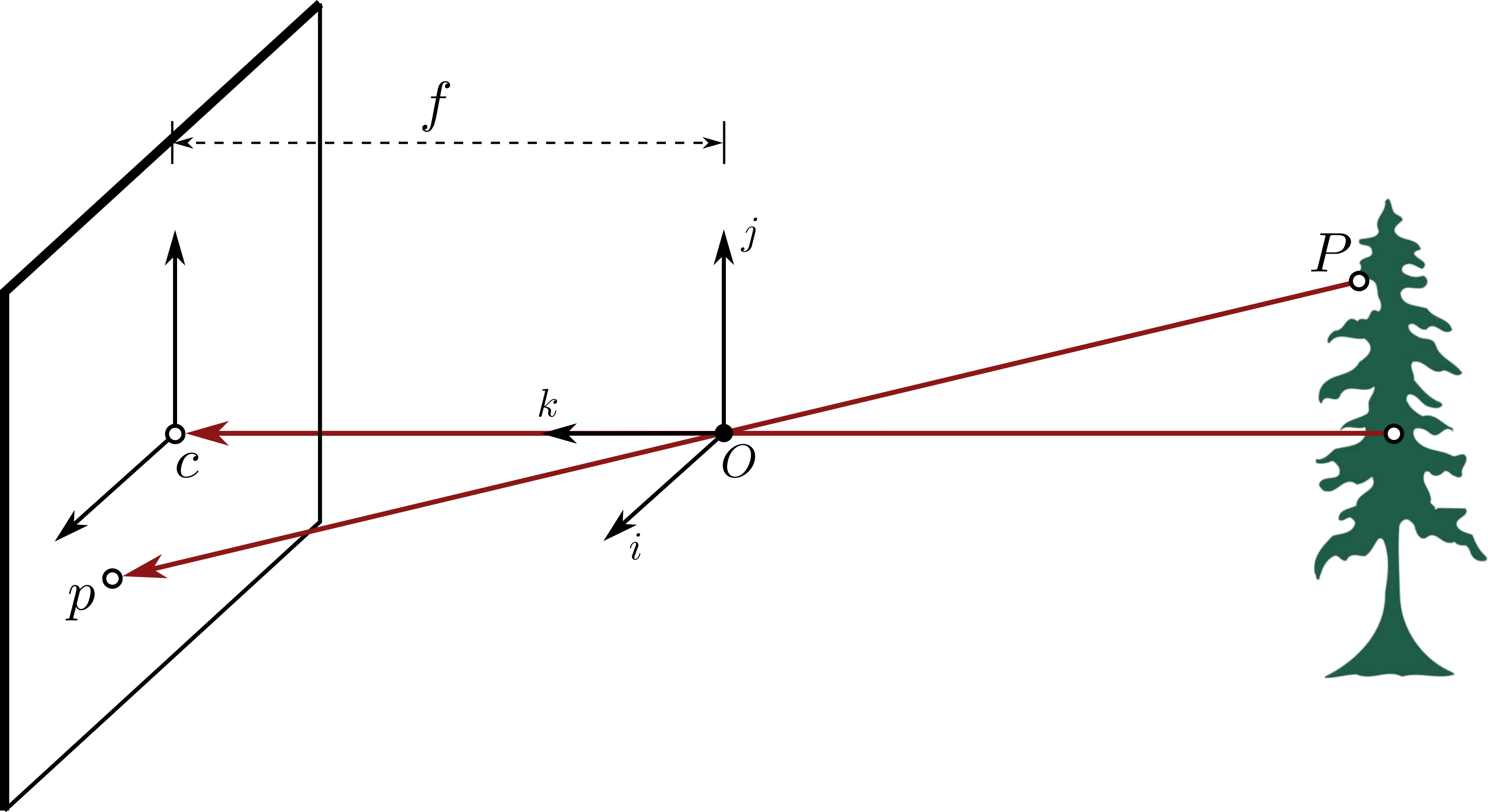
We start by defining several useful references to help develop the mathematical pinhole camera model. First, the camera reference frame is centered at a point, $O$, that is at a focal length, $f$, in front of the image plane, as we show in Figure 6.2. We define this reference frame, with directions $(i,j,k)$, such that the $k$ axis is coincident with the optical axis that points toward the image plane. We denote the coordinates of a point in the camera frame by $P=(X,Y,Z)$. When a ray of light is emitted from a point, $P$, and passes through the pinhole at point $O$, it gets captured on the image plane at a point $p$. Since these points are all collinear, we can deduce the following relationships between the coordinates $P=(X,Y,Z)$ and $p=(x,y,z)$:

$$x=\lambda X,y=\lambda Y,z=\lambda Z,$$

for some $\lambda \in ℝ$. This leads to the relationship:

$$\lambda =\frac{x}{X}=\frac{y}{Y}=\frac{z}{Z}.$$

From the geometry of the camera, we can see that $z=f$ where $f$ is the focal length, such that we can rewrite these expressions as:

$$x=f\frac{X}{Z},y=f\frac{Y}{Z}.$$

(6.1)

Therefore, we can compute the position of the pixel on the image plane that captures a ray of light from the point $P$.

One of the main issues with having a fixed pinhole aperture is that there is a trade-off associated with the aperture’s size. A large aperture allows a greater number of light rays to pass through, which leads to image blurring. A small aperture lets through fewer light rays, but the resulting image is darker. As a solution, lenses focus light by refraction and can be used to replace the aperture, avoiding the need for these trade-offs.

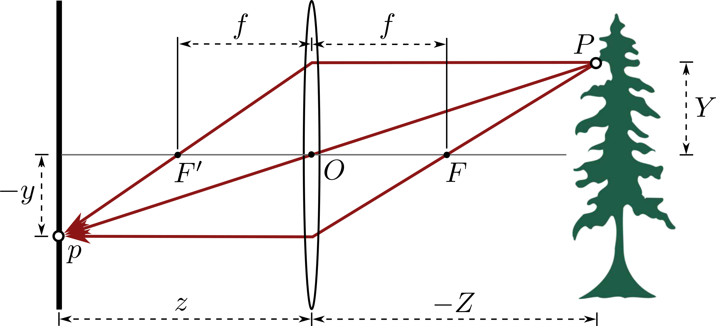
We can develop a mathematical model for lenses similar to the pinhole model by using properties from Snell’s law. Figure 6.3 shows a diagram of the most basic lens model, which is the thin lens model^††margin: The thin lens model assumes no optical distortion due to the curvature of the lens. . Snell’s law states that rays passing through the center of the lens are not refracted, and those that are parallel to the optical axis are focused on the focal point, labeled $F^{\prime }$. In addition, all rays passing through $P$ are focused by the thin lens on the point $p$. We develop a mathematical model similar to Equation 6.1 from the geometry of similar triangles:

$$\frac{y}{Y}=\frac{z}{Z},\frac{y}{Y}=\frac{z-f}{f}=\frac{z}{f}-1,$$

(6.2)

where again the point $P$ has coordinates $(X,Y,Z)$, its corresponding point, $p$, on the image plane has coordinates $(x,y,z)$, and $f$ is the focal length. Combining these two equations yields the thin lens equation:

$$\frac{1}{z}+\frac{1}{Z}=\frac{1}{f}.$$

(6.3)

Note that in this model, and for a particular focal length, $f$, a point, $P$, is only in sharp focus if the image plane is located a distance $z$ from the lens. In practice, an acceptable focus is possible within some range of distances referred to as depth of field or depth of focus. Additionally, if $Z$ approaches infinity, light would focus a distance of $f$ away from the lens. Therefore, this model is essentially the same as a pinhole model if the lens is focused at a distance of infinity.

The pinhole camera model provides a nominal camera model for which it is relatively straightforward to develop a mathematical model of the perspective projection. However, in practice, this model is not a perfect representation of the imaging process. One effect that is not captured by the pinhole model is radial distortion, which is an effect seen in real lenses where either barrel distortion or pincushion distortion will affect the real pixel coordinates. We show images of barrel and pincushion distortion in Figure 6.4.

There are methods we can use to correct for image distortion. A simple and efficient way is to model the relationship between the ideal pixel coordinates, $(u,v)$, and the distorted pixel coordinates, $(u_d,v_d)$, as:

$$\left[\begin{array}{c}{u}_d\\ v_d\end{array}\right]=(1+k{r}^2)\left[\begin{array}{c}u-u_{cd}\\ v-v_{cd}\end{array}\right]+\left[\begin{array}{c}{u}_{cd}\\ v_{cd}\end{array}\right],$$

(6.4)

where $k\in ℝ$ is the radial distortion factor, $(u_{cd},v_{cd})$ are the pixel coordinates of the image center, and $r^2={(u-u_{cd})}^2+{(v-v_{cd})}^2$ is the square of the distance between the ideal pixel location and the center of distortion. Note that $k$ differs across cameras and needs to be predetermined through calibration.

RGB-D cameras employ various technologies to capture depth information alongside color:

RGB-D cameras have enabled significant advances in several robotics applications, particularly in structured indoor environments. For indoor navigation and mapping, RGB-D sensors are ideal when GPS is unavailable and lighting can be controlled. They provide dense 3D point clouds at frame rate, enabling real-time obstacle avoidance and map building, with popular SLAM systems like RGB-D SLAM and ElasticFusion leveraging these sensors for creating detailed 3D maps. In object manipulation tasks, RGB-D cameras excel by providing both the object’s appearance and its precise 3D geometry, allowing robots to identify objects using color and texture while planning grasps based on accurate depth information. The relatively high accuracy at close range (typically 0.5 to 4 m) makes them well-suited for tabletop manipulation and pick-and-place operations.

However, several practical considerations limit their use. Most consumer RGB-D sensors operate effectively only between 0.5 and 5 meters, with accuracy degrading quadratically with distance—millimeter accuracy at one meter may degrade to several centimeters at maximum range. Material properties significantly affect performance: transparent and highly reflective surfaces cannot be measured, while dark materials may return weak signals leading to missing depth values. RGB-D cameras also require careful calibration between the color and depth sensors, which are typically offset from each other, and factory calibration may not suffice for high-precision applications. Additionally, multiple RGB-D cameras can interfere with each other’s IR projectors, and ambient infrared light (such as sunlight) makes outdoor use challenging. Despite these limitations, RGB-D cameras offer an attractive balance of cost, size, and capability for many indoor robotics applications, providing rich 3D perception without the computational complexity of stereo matching or the cost of laser scanners.

The first step we consider is how to map a point in the scene expressed in camera frame coordinates, $P_C$, to the corresponding point on the image plane, $p$, using the pinhole camera model. In the referenced item, we presented the pinhole camera equations:

$$x=f\frac{X_C}{Z_C},y=f\frac{Y_C}{Z_C},$$

(6.5)

where $P_C=(X_C,Y_C,Z_C)$, $p=(x,y)$, and $f$ is the focal length of the pinhole camera^††margin: We generally do not include the $z$ term of $p$ simply because $z=f$ is a fixed value. .

Note that the quantities $x$ and $y$ are coordinates in the camera frame, but it is often desirable to express the point $p$ in terms of pixel coordinates. Pixel coordinates are generally defined with respect to a reference frame in the lower corner of the image plane to avoid negative coordinates. We show this new reference frame in Figure 6.5, where we define the image center, $c$, with coordinates $({\tilde{x}}_0,{\tilde{y}}_0)$, where $\widetilde{(\cdot )}$ is the notation we use to denote a coordinate with respect to this new reference frame.

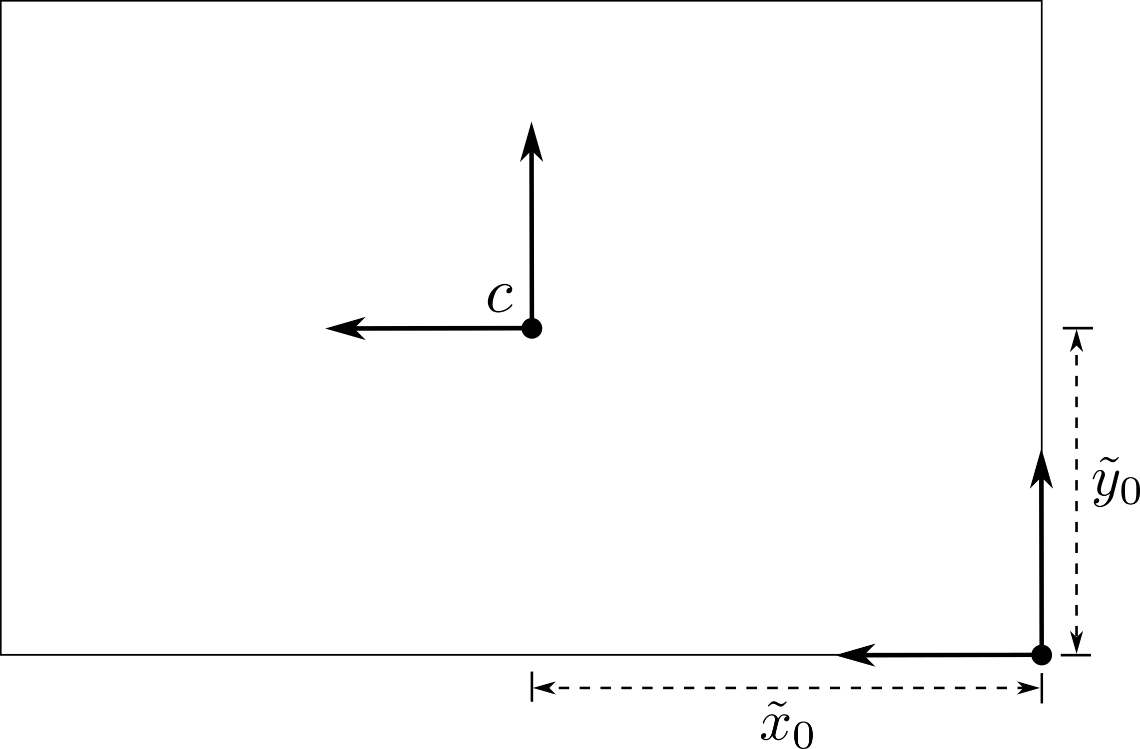
In this new reference frame, we map the point $P_C$ to the coordinates $(\tilde{x},\tilde{y})$ by:

$$\tilde{x}=f\frac{X_C}{Z_C}+{\tilde{x}}_0,\tilde{y}=f\frac{Y_C}{Z_C}+{\tilde{y}}_0.$$

(6.6)

Finally, given the number of pixels per unit distance, we can map these new coordinates to pixel coordinates. In particular, we map the point $P_C$ to pixel coordinates $(u,v)$ by:

$$u=\alpha \frac{X_C}{Z_C}+u_0,v=\beta \frac{Y_C}{Z_C}+v_0,$$

(6.7)

where $\alpha =k_{x}f$, $u_0=k_x{\tilde{x}}_0$, $\beta =k_{y}f$, $v_0=k_y{\tilde{y}}_0$, and $k_x$ and $k_y$ are the number of pixels per unit distance in image coordinates.

Note that the transformation from the point $P_C$ in camera frame coordinates to $p$ in pixel coordinates given by Equation 6.7 is not linear. However, we can represent this transformation as a linear mapping^††margin: Expressing the perspective projection as a linear map will simplify the mathematics later on. through an additional change of coordinates. In particular, we will express the points $P_C$ and $p$ in homogeneous coordinates.

For a two-dimensional point $(x_1,x_2)$ or a three-dimensional point $(x_1,x_2,x_3)$ in Euclidean space, we represent the point in homogeneous coordinates by the transformation:

$$(x_1,x_2)\to (\alpha x_1,\alpha x_2,\alpha ),\text{and}(x_1,x_2,x_3)\to (\alpha x_1,\alpha x_2,\alpha x_3,\alpha ),$$

(6.8)

for any $\alpha \ne 0$. These new coordinates are called homogeneous coordinates because we can choose the scaling factor, $\alpha$, arbitrarily as long as $\alpha \ne 0$. We transform a set of homogeneous coordinates back by:

$$(y_1,y_2,y_3)\to (\frac{y_1}{y_3},\frac{y_2}{y_3}),\text{and}(y_1,y_2,y_3,y_4)\to (\frac{y_1}{y_4},\frac{y_2}{y_4},\frac{y_3}{y_4}).$$

(6.9)

We will denote when a point is described in homogeneous coordinates using the superscript $h$. For example, we express the point $P_C=(X_C,Y_C,Z_C)$ in camera frame coordinates with $\alpha =1$ in homogeneous coordinates by:

$$P_C^h=(X_C,Y_C,Z_C,1),$$

and we can express the pixel coordinate $p=(u,v)$ in homogeneous coordinates by:

$$p^h=(Z_{C}u,Z_{C}v,Z_C)=(\alpha X_C+u_0{Z}_C,\beta Y_C+v_0{Z}_C,Z_C),$$

by choosing $\alpha =Z_C$ and substituting the expressions from Equation 6.7. With the expression of these points in homogeneous coordinates, we can see that their relationship is transformed from the nonlinear relationship in Equation 6.7 to the linear relationship:

(6.10)

Often, in practice, we also add a skewness parameter, $\gamma$^††margin: The skewness parameter generally ends up being close to zero. , and we can write this linear relationship in the more compact form:

(6.11)

We refer the matrix $K$ in Equation 6.11 as the camera matrix or matrix of intrinsic parameters because it contains the five parameters that define the fundamental characteristics of the camera from the perspective of the pinhole camera model. While these parameters may be specified by the camera manufacturer, we often estimate them in practice by performing a camera calibration.

We can express a point, $P$, in the scene (see Figure 6.2) either in terms of camera frame coordinates, $P_C$, or world frame coordinates, $P_W$. While we discussed the use of the pinhole model to map $P_C$ coordinates to pixel coordinates, $p$, in the previous section, in this section we discuss the mapping between the camera and world frame coordinates of the point $P$, as we show in Figure 6.6.

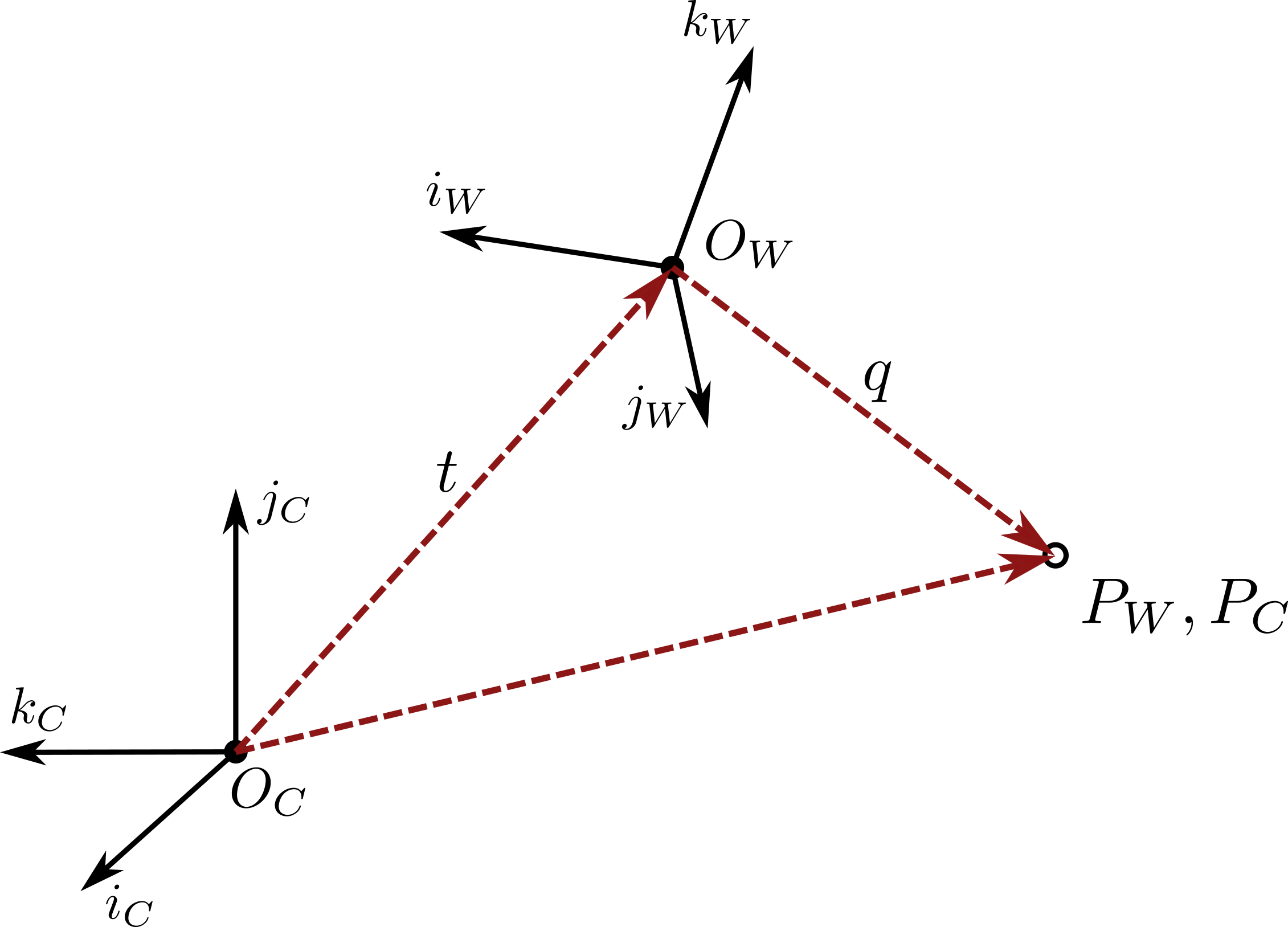
From Figure 6.6, we can write $P_C$ as:

$$P_C=t+q,$$

(6.12)

where $t$ is the vector from $O_C$ to $O_W$, expressed in camera frame coordinates, and $q$ is the vector from $O_W$ to $P$, expressed in camera frame coordinates. However, the vector $q$ is the same vector as $P_W$, just expressed with respect to a different coordinate frame. The coordinates are related by a rotation:

$$q=R{P}_W,$$

(6.13)

where $R$ is the rotation matrix relating the camera frame to world frame defined as:

(6.14)

where $i$, $j$, and $k$ are the unit vectors that define the camera frame and $i_w$, $j_w$, and $k_w$ are the unit vectors that define the world frame. To summarize, we can map the point $P_W$ to camera frame coordinates $P_C$ by:

$$P_C=t+R{P}_W,$$

(6.15)

where $t$ is the vector in camera frame coordinates from $O_C$ to $O_W$ and $R$ is the rotation matrix defined in Equation 6.14. Similar to the previous section, we can equivalently express this transformation for the case where the points $P_W$ and $P_C$ are expressed in homogeneous coordinates:

(6.16)

The objective of the perspective projection task is to find a way to mathematically relate the position of a point in world frame coordinates, denoted $P_W$, to the corresponding pixel coordinates, $p$, on the image plane. With the relationship from Equation 6.16 that we developed for mapping $P_W$ to the camera frame coordinates, $P_C$, and the relationship in Equation 6.11 for mapping $P_C$ to pixel coordinates, $p$, we can now define the direct mapping from $P_W$ to $p$. In particular, combining the two transformations together yields:

which we can simplify to:

(6.17)

In Equation 6.17, $P_W^h$ is the homogeneous coordinate representation of $P_W$ and $p^h$ is the homogeneous coordinate representation of $p$. Recall that the matrix $K\in {ℝ}^{3\times 3}$ is the matrix of intrinsic camera parameters, and the matrix $[Rt]\in {ℝ}^{3\times 4}$ contains extrinsic parameters^††margin: Extrinsic parameters describe the camera’s position and orientation relative to the points in the scene. . Note that the total number of degrees of freedom is 11, where 5 are from the intrinsic parameters that define $K$, 3 are from the rotation matrix, $R$, and 3 are from the position vector, $t$.

One approach is the direct linear calibration method, which requires a set of known correspondences, $p_i\stackrel{}{\leftrightarrow }{P}_{W,i}$ for $i=1,\mathrm{\dots },n$.

The projection matrix, $M$, is defined for a specific set of extrinsic parameters $R$ and $t$. In practice, however, it might be desirable for us to estimate the camera’s intrinsic parameters from $N$ different images from different perspectives, and therefore with $N$ different projection matrices due to the varying extrinsic parameters. In this case, we can apply an alternative procedure⁵5. Zhang, Z. “A Flexible New Technique for Camera Calibration.” IEEE Transactions on Pattern Analysis and Machine Intelligence 22, 2000. to the direct linear calibration method to extract the intrinsic parameters, $K$.

We begin by assuming that the known points, $P_W$, for each individual image lie on a plane. For example, the calibration scene might consist of a pattern, such as a checkerboard pattern, on a planar surface. In this case, we can assume that the world frame origin lies on the plane such that $Z_W=0$ for all points on the plane. Since $Z_W=0$, we can simplify the relationship between $p^h$ and $P_W^h$ given by Equation 6.17 to:

$$p^h=H{\tilde{P}}_W^h,$$

(6.26)

with:

(6.27)

where $H$ is called the homography matrix^††margin: The homography matrix maps points between two-dimensional planes while a projection matrix maps three-dimensional points to points on a two-dimensional plane. , ${\tilde{P}}_W^h$ is the simplified position of the point $P$ in world frame, written in homogeneous coordinates, and $r_i$ is the $i$-th column of the rotation matrix, $R$. Note that we can still estimate the homography matrix, $H$, using the same procedure discussed earlier.

Next, we identify a set of constraints on the intrinsic parameter matrix, $K$, by writing the homography, $H$, as:

and noting that since $r_1$ and $r_2$ are orthonormal we have:

$${\tilde{c}}_1^{\top }B{\tilde{c}}_2=0,{\tilde{c}}_1^{\top }B{\tilde{c}}_1={\tilde{c}}_2^{\top }B{\tilde{c}}_2,$$

(6.28)

where $B=K^{-\top }{K}^{-1}\in {ℝ}^{3\times 3}$ is a symmetric matrix. We can therefore solve for the intrinsic camera parameters, $K$, by using the constraints in Equation 6.28 to solve for the symmetric matrix $B$ and then backing out the parameters that define $K$. To compute the matrix $B$ from the constraints in Equation 6.28, we can employ several useful tricks. The main trick is to notice that even though $B$ consists of nine parameters, it is symmetric, and, therefore, we only need six parameters to specify it fully. Therefore, we reparameterize the matrix $B\in {ℝ}^{3\times 3}$ as a vector $b\in {ℝ}^6$ as:

(6.29)

This reparameterization is useful because it allows us to rewrite the expression ${\tilde{c}}_i^{\top }B{\tilde{c}}_j$ as:

$${\tilde{c}}_i^{\top }B{\tilde{c}}_j=v_{ij}^{\top }b,$$

(6.30)

where:

and where ${\tilde{c}}_{ik}$ is the $k$-th element of the column vector ${\tilde{c}}_i$ and ${\tilde{c}}_{jk}$ is the $k$-th element of the column vector ${\tilde{c}}_j$. With this reparameterization, we can rewrite the constraints in Equation 6.28 as:

or by combining them:

$$\left[\begin{array}{c}{v}_{12}^{\top }\\ {(v_{11}-v_{22})}^{\top }\end{array}\right]b=0,$$

(6.31)

which is linear with respect to the unknowns vector $b$. Importantly, while the homographies, $H$, are different for each image due to the different extrinsic parameters, the intrinsic camera parameters represented by the vector $b$ are the same. Therefore, with $N$ images from the same camera, even with potentially different perspectives, we can stack the constraints in Equation 6.31 to give:

$$Vb=0,$$

(6.32)

where $V\in {ℝ}^{2N\times 6}$. In the case where we include the skewness parameter, $\gamma$, in $K$, there must be $N\ge 3$ images in order to specify $B$ uniquely. Similarly to the approach for computing the projection matrix in the previous section, we can compute the vector $b$ as the solution to the constrained least squares problem:

(6.33)

Once we have computed $b$, we can solve for the intrinsic camera parameters, $K$, by leveraging the definition of $B=K^{-T}{K}^{-1}$. In particular, we compute the intrinsic parameters by:

(6.34)

where we can think of $\lambda$ as a scaling parameter that accounts for the fact that there are five unknown camera intrinsic parameters but six degrees of freedom in $B$.

Once we have extracted the camera intrinsic parameters, $K$, from this procedure, given any new homography, $H$, we can compute the extrinsic parameters by:

(6.35)

As one final step, we note that the matrix $R$ defined with column vectors $r_1$, $r_2$, and $r_3$ will not generally satisfy the orthonormality property of a rotation matrix. We can correct this issue by again using optimization methods to compute a valid rotation matrix that best corresponds to these column vectors:

(6.36)

where:

We solve this problem by choosing $R=U{V}^{\top }$, where $U$ and $V$ are defined by the singular value decomposition of $Q=U\mathrm{\Sigma }{V}^{\top }$.

The direct linear transformation from Section 6.5.1 and Zhang’s flexible calibration method from Section 6.5.2 require point correspondences to calculate the intrinsic and extrinsic parameters. Auto-calibration offers an alternative approach that does not make this assumption by utilizing multiple views of a static scene to determine the camera’s intrinsic and extrinsic parameters. This approach leverages the fact that a camera’s intrinsic parameters remain constant across different views of the same scene. By identifying correspondences between points in multiple images, we can estimate the intrinsic matrix, $K$, and extrinsic matrices, $R$ and $t$, by bundle adjustment based on the static scene geometry. In total, the camera auto-calibration process consists of five key steps.

First, we use an algorithm such as scale-invariant feature transform (SIFT) to identify key points in the scene and their correspondence points across multiple images from different views. The SIFT algorithm is a computer vision method to detect, describe, and match local features in images. It is robust in detecting and describing local features in images, making it effective for finding correspondences under varying conditions. Details of the SIFT algorithm will be discussed in the following chapters.

Second, we use the correspondences between a pair of images to compute the fundamental matrix. The fundamental matrix, $F\in {ℝ}^{3\times 3}$, relates corresponding points between a pair of images of the same scene^††margin: The fundamental matrix describes the epipolar geometry between two image views. . For a pair of images $(I,I^{\prime })$ of the same scene, the fundamental matrix, $F$, satisfies:

$$p^{\top }F{p}^{\prime }=0,$$

(6.37)

where $p$ and $p^{\prime }$ are corresponding points in images $I$ and $I^{\prime }$, respectively. We will discuss the fundamental matrix more in the context of stereo vision in Chapter 7.

To compute the fundamental matrix for the image pair, we first construct a point correspondence matrix, $W$, where each row represents a correspondence between points in the two images. Let $(u_i,v_i)$ and $(u_i^{\prime },v_i^{\prime })$ be the coordinates of one set of matched points, $p_i$ and $p_i^{\prime }$. We form each row of the matrix $W$ using one set of corresponding coordinates as:

(6.38)

From this point correspondence matrix, we then compute the fundamental matrix by solving the linear system $Wf=0$ using a singular value decomposition (SVD), where $f$ is the vectorized form of the fundamental matrix. We describe the specifics of this procedure in more detail in the referenced item.

Third, we compute the essential matrix, which is similar to the fundamental matrix in that it relates corresponding points in two images based on scene geometry. For two images, $I$ and $I^{\prime }$, we define the essential matrix by the rotation matrix, $R$, and translation vector, $t$, relating the coordinate frames of the two images by:

$$E={[t]}_{\times }R,$$

(6.39)

where ${[t]}_{\times }$ is the matrix representation of the cross product. Assuming the intrinsic matrix, $K$, remains the same between the images, we can also define the essential matrix, $E$, with respect to the fundamental matrix as:

$$E=K^{\top }FK.$$

(6.40)

Therefore, we can first compute the essential matrix from the previously computed fundamental matrix and the intrinsic parameter matrix, $K$, and then we can compute the camera extrinsic rotation and translation parameters, $R$ and $t$, by the singular value decomposition:

$$E=U\mathrm{\Sigma }{V}^{\top },$$

(6.41)

where $\mathrm{\Sigma }=\text{diag}(1,1,0)$. From this decomposition, there are two possible solutions for the camera extrinsic parameters:

	$R_1$	$=UW{V}^{\top },$	$R_2$	$=U{W}^{\top }{V}^{\top },$		(6.42)
	$t_1$	$=U[:,2],$	$t_2$	$=-U[:,2],$

where:

(6.43)

We can identify the correct solution by using each to compute the three-dimensional points from the two-dimensional matched correspondence points, as we describe in the next step. The extrinsic parameters, $R$ and $t$, we should use are the ones that ensure that most of the three-dimensional points lie in front of both cameras, meaning they will have positive depth values.

The fourth step is to perform triangulation to compute the 3D points in the scene from the 2D image correspondence points. We define the projection matrix, $P$, for an image as:

(6.44)

where again $K$ is the camera intrinsic matrix, $R$ is the rotation matrix, and $t$ is the translation vector. This projection matrix maps a 3D point in homogeneous coordinates into the 2D camera frame coordinates by:

$$\left[\begin{array}{c}u\\ v\\ 1\end{array}\right]=P\left[\begin{array}{c}X\\ Y\\ Z\\ 1\end{array}\right].$$

(6.45)

Therefore, for matched points across two images, we can compute the 3D coordinates by solving the linear system:

$$\left[\begin{array}{c}u{P}_3^{\top }-P_1^{\top }\\ v{P}_3^{\top }-P_2^{\top }\\ u^{\prime }{P}_3^{\prime \top }-P_1^{\prime \top }\\ v^{\prime }{P}_3^{\prime \top }-P_2^{\prime \top }\end{array}\right]\left[\begin{array}{c}X\\ Y\\ Z\\ 1\end{array}\right]=0,$$

(6.46)

where $(u,v)$ are the coordinates and $P_1$, $P_2$, and $P_3$ are the first, second, and third rows of the projection matrix, $P$, for image $I$, respectively, and $(u^{\prime },v^{\prime })$ are the coordinates and $P_1^{\prime }$, $P_2^{\prime }$, and $P_3^{\prime }$ are the rows of the projection $P^{\prime }$ for image $I^{\prime }$. We can solve Equation 6.46 using a least squares method.

So far, we have used correspondences in pairs of images from the same camera of the same scene to estimate the image extrinsics, $R$ and $t$, and computed estimates of the 3D scene points by triangulation. These computations require knowledge of the camera intrinsic matrix, $K$, which is the quantity we are trying to estimate. We can leverage the previous steps to compute $K$ by using an iterative optimization-based procedure, where we begin with an estimate^††margin: For example, we could start with an estimate by referencing the camera manufacturer’s data, or using some other simpler method. of $K$ and refine it until convergence. In particular, we refine the estimate of the camera intrinsics and extrinsics by solving the optimization:

$$\sum _{i=1}^N\sum _{j=1}^M{\Vert p_{ij}-P_i(K,R_i,t_i)X_j\Vert }^2,$$

(6.47)

where $p_{ij}$ is an observed 2D point in image $i$ that corresponds to the $j$-th 3D point, $X_j$ is the $j$-th estimated 3D point, $P_i(K,R_i,t_i)$ is the projection matrix for image $i$, $M$ is the total number of triangulated 3D points, and $N$ is the total number of images. Note that each projection matrix is a function of the intrinsic parameters, which are constant across all images, as well as the extrinsic parameters for the image. We can optimize this cost function by applying a nonlinear method, such as Levenberg-Marquardt, to compute a new set of parameters. We then repeat the steps listed above, computing new extrinsics, triangulation points, and optimizing, until convergence.