In Chapter 6, we introduced the mathematical relationship between the position of a point, , in a scene, expressed in world frame coordinates, , and the corresponding point, , in pixel coordinates that gets projected onto the image plane of a camera. This relationship is based on the pinhole camera model, and requires knowledge about the camera’s intrinsic and extrinsic parameters. We also presented methods for camera calibration, which allow us to determine these parameters. Given a calibrated camera with known parameters, a fundamental problem in robotic perception is how to leverage images to recover three-dimensional information about the structure of the environment††margin: While we could use other sensors to recover three-dimensional scene information, such as ultrasonic sensors or laser rangefinders, cameras capture a broad range of information that goes beyond depth sensing and are attractive based on their cost and size. . The camera projection model alone does not provide us with enough information to fully determine the 3D position of a point from a single image, specifically because we cannot determine the point’s depth††margin: Unless you are willing to make strong assumptions, for example that you know the physical dimensions of the objects in the environment. .
In this chapter, we introduce stereo vision in Section 7.1 and structure from motion in Section 7.3, two approaches for extracting 3D information from camera images. Both leverage multiple images of a scene to determine three-dimensional structure: stereo vision uses images from different viewpoints captured simultaneously by two or more cameras, while structure from motion uses images captured sequentially from a single moving camera. These techniques form the visual foundation for many robotic applications including navigation, mapping, and manipulation.
7.1 Stereo Vision
Stereopsis††margin: From stereo, meaning solidity, and opsis, meaning vision or sight. is the process in visual perception leading to the sensation of depth from two slightly different projections of the world onto the retinas of the two eyes. The difference in the two retinal images is called horizontal disparity, retinal disparity, or binocular disparity, and arises from our eyes’ different positions in the head. This disparity enables our brain to fuse the two retinal images into a single percept with depth information. For example, if you hold your finger vertically in front of you and alternate closing each eye, you will see that the finger jumps from left to right—this lateral displacement is the disparity between your eyes.
Computational stereopsis, or stereo vision, is the process of obtaining depth information from images captured by two or more cameras observing the same scene from different perspectives. This process consists of two major steps: fusion and reconstruction. Fusion involves solving the correspondence problem—identifying which pixels in each image correspond to the same 3D point. Reconstruction uses these correspondences to triangulate the 3D position of scene points, including their depth.
7.1.1 Epipolar Geometry
The first step in stereo vision is to establish correspondences between images††margin: We generally assume that the perspectives differ only slightly, such that features appear similar across images. . This task can be challenging, as incorrect matches lead to large reconstruction errors. Epipolar geometry provides powerful constraints that simplify correspondence search and improve matching accuracy.
Epipolar constraints.
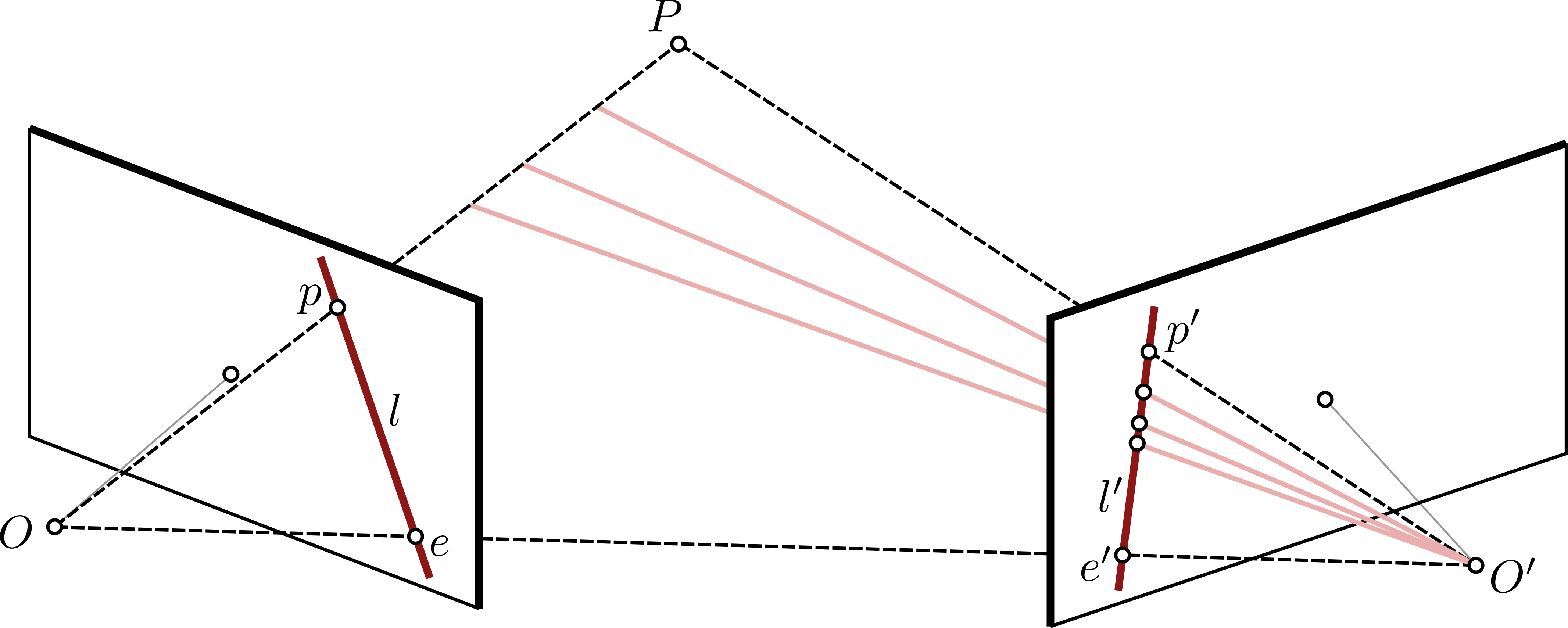
Consider the image projections and of a scene point observed by two cameras with optical centers and , as shown in Figure 7.1. These five points all lie in the epipolar plane, defined by the two rays and . The intersection of this plane with each image plane forms the epipolar lines and , which pass through the epipoles and —the projections of each camera center onto the other camera’s image plane. This geometric relationship provides a powerful constraint: if and are projections of the same point , then must lie on epipolar line and must lie on epipolar line . This epipolar constraint reduces the correspondence search from a two-dimensional problem to a one-dimensional search along epipolar lines. Mathematically, we express this constraint using the coplanarity of the vectors:
| (7.1) |
Fundamental and essential matrices.
When the world reference frame coincides with the first camera’s frame (origin at ), we can express the epipolar constraint as:
| (7.2) |
where is the fundamental matrix. The fundamental matrix encodes the epipolar geometry between two views and has seven degrees of freedom (it is defined up to scale and has rank 2). It depends only on the cameras’ intrinsic parameters and their relative pose:
| (7.3) |
where and are the intrinsic parameter matrices for the two cameras, and is the essential matrix:
| (7.4) |
with and being the rotation and translation that transform points from the second camera frame to the first.
The fundamental matrix also defines the epipolar lines: and . The epipoles satisfy and , confirming that is singular (rank 2). To estimate from image correspondences, we use the fact that each correspondence provides one linear constraint. With and in homogeneous coordinates, we can rewrite the epipolar constraint as:
| (7.5) |
where is the vectorized form of . Given correspondences, we stack these constraints into a matrix equation and solve:
| (7.6) |
The solution is the eigenvector corresponding to the smallest eigenvalue of . Since the resulting matrix may not have rank 2, we enforce the singularity constraint by computing the SVD of and setting the smallest singular value to zero.
Image rectification.
Epipolar rectification transforms stereo image pairs such that epipolar lines become horizontal and aligned across images. This transformation simplifies correspondence search to a one-dimensional problem along image rows, significantly reducing computational cost. The rectified configuration is equivalent to having two cameras with parallel optical axes and aligned image rows, separated by a baseline distance.
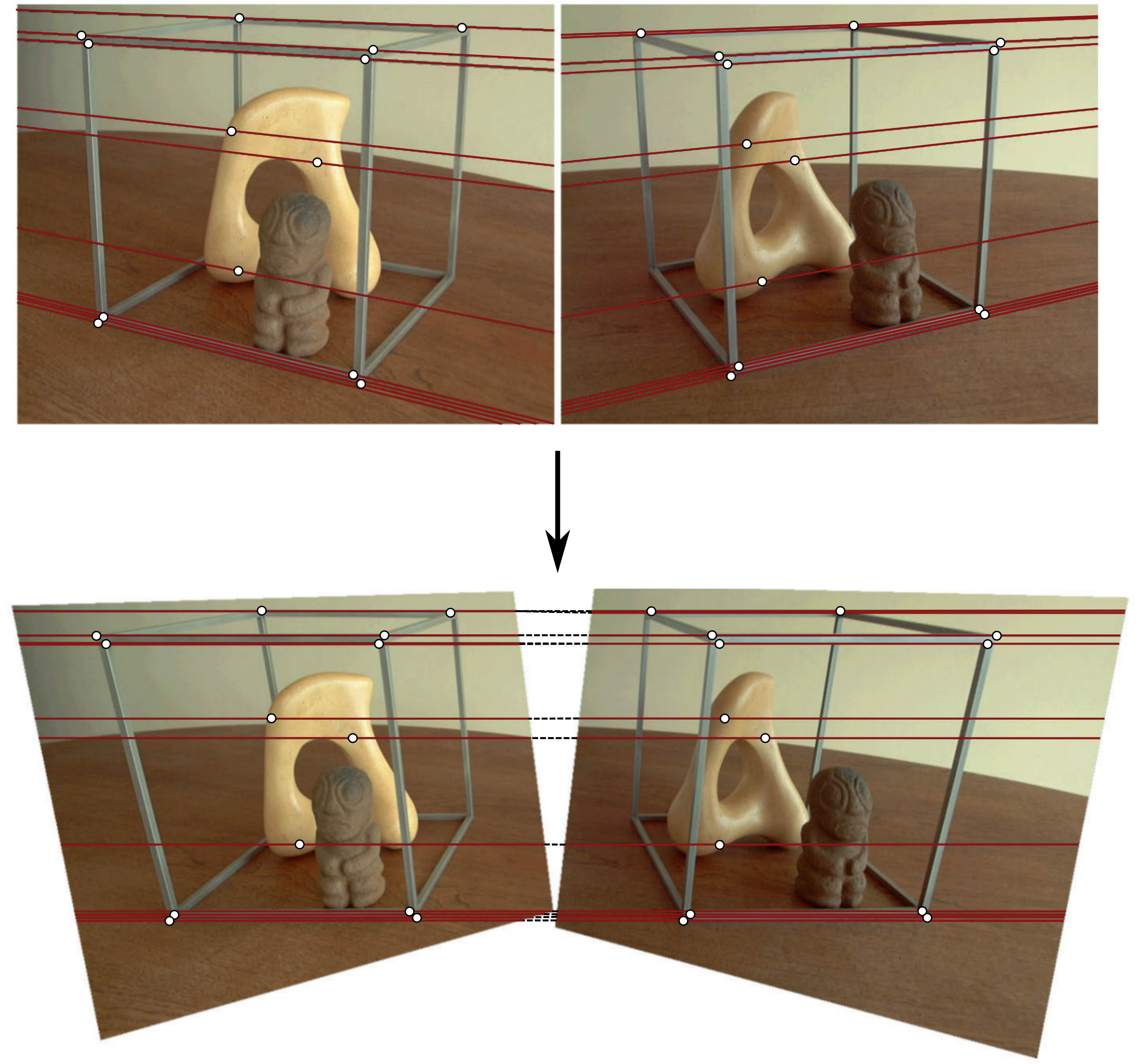
After rectification, as shown in Figure 7.2, correspondence search is constrained to horizontal scan lines, making stereo matching algorithms more efficient and robust.
7.2 Correspondence and Reconstruction
With the geometric constraints established through epipolar geometry and simplified through image rectification, we now turn to the practical challenges of stereo vision. The correspondence problem—determining which pixels in each image represent the same scene point—remains the most critical and challenging step, as errors here propagate directly to the reconstructed 3D structure. Once reliable correspondences are found, triangulation transforms these matched points into 3D coordinates, with the accuracy depending fundamentally on the system geometry and image measurements.
The correspondence problem.
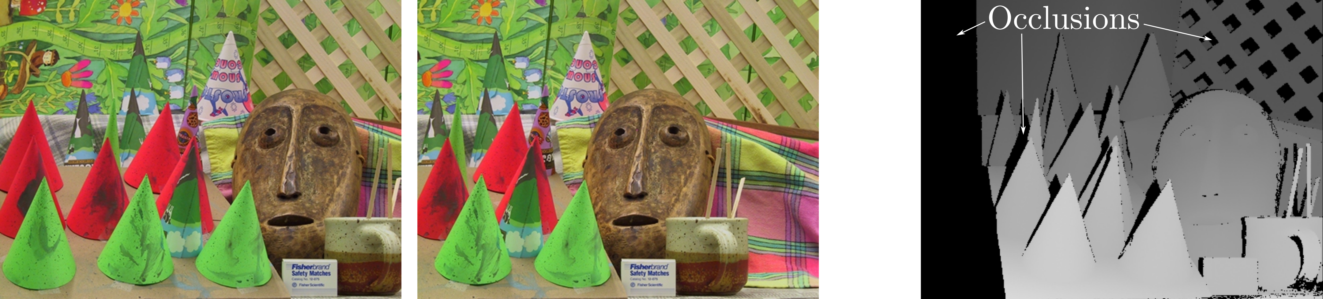
Even with epipolar constraints and rectification, finding correct correspondences remains challenging. Occlusions occur when points visible in one view are hidden in another, while repetitive patterns in textured regions create ambiguous matches where multiple locations appear identical. Conversely, uniform regions lack sufficient texture for reliable feature matching, and perspective distortions cause features to appear different across viewpoints despite representing the same scene point. Modern stereo matching algorithms address these challenges through robust feature descriptors, correlation-based matching over local windows, or learned representations that capture scene semantics beyond low-level appearance.
Triangulation and disparity.
Once correspondences are established, we reconstruct 3D points through triangulation. For rectified stereo pairs with parallel optical axes separated by baseline , the geometry simplifies considerably, as shown in Figure 7.3.
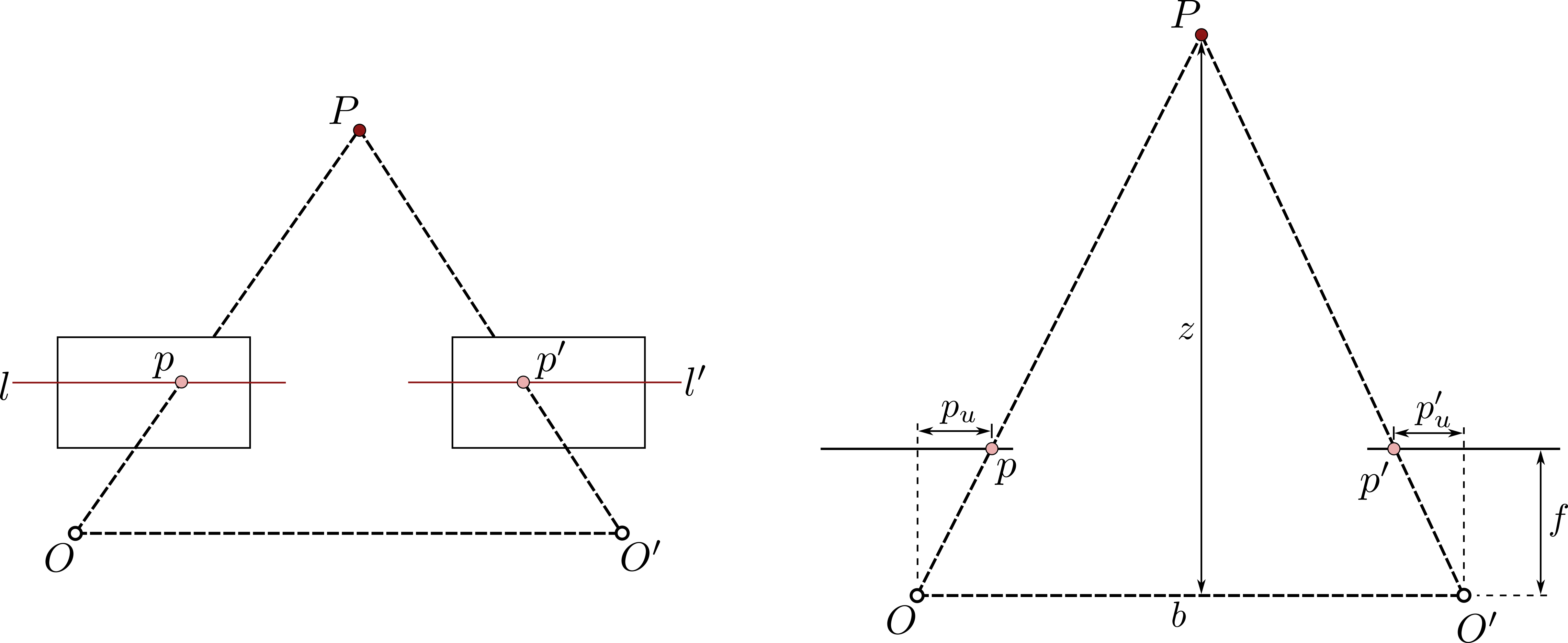
From similar triangles, we derive the fundamental stereo equation:
| (7.7) |
where is depth, is baseline, is focal length, and is the disparity—the difference in horizontal coordinates between corresponding points.
This inverse relationship between depth and disparity has important implications for stereo system design. Near objects produce large disparities and thus accurate depth estimates, while distant objects yield small disparities with correspondingly less accurate depth measurements. Since depth resolution decreases quadratically with distance, baseline selection becomes critical: larger baselines improve depth accuracy for distant objects but increase occlusions where one camera cannot see points visible to the other. This fundamental trade-off must be considered when designing stereo systems for specific applications.
Disparity maps.
A disparity map encodes the disparity value for each pixel, providing a dense depth representation of the scene. Figure 7.4 shows an example where brighter regions indicate larger disparities (closer objects) and black regions represent occluded areas where no correspondence exists. Dense disparity estimation extends the correspondence problem from sparse feature matching to every pixel, requiring additional regularization to handle ambiguous regions while preserving depth discontinuities at object boundaries.
7.3 Structure From Motion
The structure from motion (SFM) method uses a similar principle as stereo vision, but uses a single camera to capture multiple images from different perspectives while moving within the scene. In this case, the intrinsic camera parameter matrix, , will be constant across images, but the extrinsic parameters consisting of the rotation matrix, , and relative position vector, , will be different for each image.
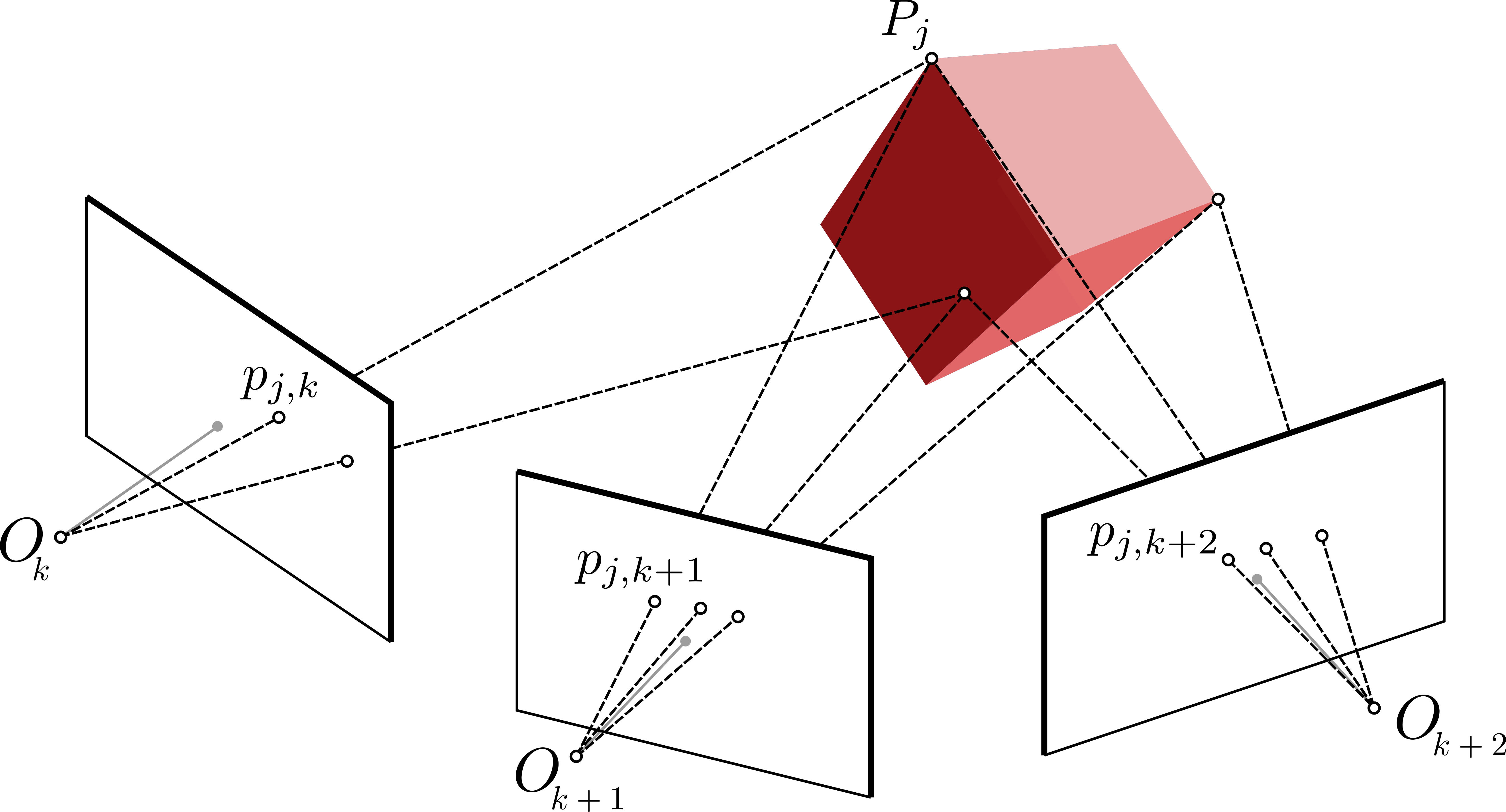
Consider a case where we take images of fixed 3D points from different perspectives. This would lead to projection matrices, , and 3D points, , that we would need to determine by leveraging the projection relationships:
Notice that there is quite a bit of similarity between this problem and the camera auto-calibration problem discussed in Chapter 6, except here we assume we already know the camera intrinsic parameters.
The fundamental challenge in structure from motion is to simultaneously recover both the camera poses and the 3D point positions from only the 2D image observations. This requires solving a large optimization problem with many unknowns, which we approach either incrementally by adding one image at a time, or globally by considering all images simultaneously. Both approaches rely on establishing feature correspondences across images and minimizing reprojection errors through bundle adjustment. Structure from motion methods also have some unique limitations. Most notably, there exists an inherent ambiguity in the absolute scale of the scene that cannot be determined from images alone††margin: For example, a bigger object at a longer distance and a smaller object at a closer distance can yield identical projections. . Additionally, errors accumulate over long sequences, leading to drift that must be corrected through loop closure when the camera revisits a previous location. Despite these challenges, structure from motion has proven invaluable for robotic applications where carrying multiple cameras is impractical.
7.3.1 Two-View Geometry
The structure from motion pipeline begins with reconstructing the scene from two views, establishing the initial geometry that subsequent images will extend. Given correspondences between two images taken from positions and , we first estimate the fundamental matrix using the same techniques described for stereo vision. With known intrinsics, we recover the essential matrix and decompose it to obtain the relative camera pose.
The decomposition of the essential matrix yields four possible solutions for the rotation and translation . We identify the correct solution by verifying that reconstructed points have positive depth in both camera views. Once the relative pose is established, we triangulate the matched features to obtain initial 3D points. For each correspondence , the 3D point satisfies:
| (7.8) |
where and are the projection matrices for cameras at and , and denotes the skew-symmetric matrix formed from the homogeneous coordinates of . This linear system is solved using least squares, typically with singular value decomposition for numerical stability.
7.3.2 Sequential Reconstruction
Sequential structure from motion extends the initial two-view reconstruction by incrementally incorporating new images, as illustrated in Figure 7.5. Each new image captured from position undergoes pose estimation through perspective-n-point (PnP) solving, which finds the camera position that minimizes reprojection error for correspondences between image points and existing 3D points . Once registered, the image contributes new scene points through triangulation with previously registered views from positions .
The critical challenge is maintaining consistency as errors accumulate. Bundle adjustment jointly optimizes camera poses and 3D points to minimize total reprojection error:
| (7.9) |
where represents the observed projection of point in the image taken from camera position , and denotes the set of points visible from viewpoint . However, global optimization after each image is computationally prohibitive. Instead, we perform local bundle adjustment over a sliding window of recent images (typically spanning positions through ), maintaining local accuracy while deferring global consistency to a final optimization step. This windowed approach achieves near-global accuracy at a fraction of the computational cost, making the method practical for long image sequences. Image selection order also affects reconstruction quality—we typically choose the next viewpoint that maximizes correspondences with the current reconstruction, balancing accurate pose estimation with effective triangulation of new points.
Global structure from motion.
An alternative to sequential reconstruction is global structure from motion, which estimates all camera poses simultaneously before triangulating points. This approach first constructs an epipolar graph connecting all image pairs with sufficient matches, then solves for all rotations and translations globally through rotation and translation averaging. While potentially more accurate than incremental methods, global approaches require solving large optimization problems and may be less robust to outliers in practice. The choice between sequential and global methods often depends on the specific application requirements and computational resources available.
7.3.3 Visual Odometry
One particularly important application of the structure from motion concept is visual odometry, which estimates robot motion in real-time using visual input. Visual odometry prioritizes speed and local accuracy over global consistency, maintaining only a sliding window of recent frames and performing limited bundle adjustment. This approach operates at camera frame rates by trading global optimality for computational efficiency. Visual odometry has proven invaluable for robot navigation, particularly in environments where wheel odometry is unreliable or unavailable. Mars rovers, for instance, rely on visual odometry to navigate terrain where wheel slip would cause traditional odometry to fail dramatically††margin: The Mars Exploration Rovers Spirit and Opportunity used stereo visual odometry to traverse over 45 kilometers combined, far exceeding their planned 600-meter missions. . The technique also enables navigation for flying robots and underwater vehicles where wheel odometry is impossible.
Modern visual odometry systems often combine multiple approaches for robustness. Feature-based methods track distinctive image features across frames, providing robustness to illumination changes but potentially failing in textureless environments. Direct methods minimize photometric error using raw pixel intensities, exploiting all image information but requiring good initialization and small inter-frame motions. Hybrid approaches leverage the strengths of both, using features for robustness and direct alignment for accuracy.
7.3.4 Loop Closure and Drift Mitigation
Over extended sequences, small errors in structure from motion accumulate into significant drift. Loop closure detection identifies when the camera revisits a previous location, providing constraints to correct this accumulated error globally. This involves recognizing previously seen places despite changes in viewpoint and lighting, typically using visual vocabularies or learned features, followed by geometric verification and global optimization incorporating the loop constraints. Successfully detecting and closing loops transforms structure from motion from a local reconstruction technique into a method capable of mapping large environments—a capability essential for autonomous navigation.
7.4 Summary
This chapter presented two fundamental approaches for extracting 3D information from camera images. Stereo vision leverages simultaneous views from multiple cameras, using epipolar geometry to constrain correspondence search and enable real-time depth estimation through triangulation. Structure from motion reconstructs scene geometry from sequential images captured by a moving camera, trading real-time performance for the flexibility of a single-camera system. Both techniques face similar challenges—establishing correspondences between images despite occlusions, repetitive textures, and perspective distortions. The reconstruction accuracy depends fundamentally on baseline configuration: stereo systems use fixed baselines while structure from motion adapts its effective baseline through camera motion. However, structure from motion suffers from scale ambiguity that must be resolved through additional sensors or known scene dimensions. These complementary approaches have enabled numerous robotic applications, from Mars rover navigation using visual odometry to autonomous vehicle perception using stereo depth. Modern systems increasingly combine both techniques with other sensors—visual-inertial odometry fuses structure from motion with IMU data to recover metric scale, while stereo visual odometry leverages multiple cameras with motion estimation for robust navigation.
To learn more.
For a comprehensive treatment of stereo vision and structure from motion, including advanced algorithms and practical implementations, readers are encouraged to consult the textbooks Introduction to Autonomous Mobile Robots by Siegwart et al. (2011)11. Siegwart, R., Nourbakhsh, I. R., Scaramuzza, D. Introduction to Autonomous Mobile Robots. MIT Press, 2011. and Computer Vision: A Modern Approach by Forsyth and Ponce (2011)22. Forsyth, D. A., Ponce, J. Computer Vision: A Modern Approach. Prentice Hall, 2011.. Additionally, for a deeper understanding of epipolar geometry and multi-view reconstruction, readers can refer to the works Fusiello et al. (2000)33. Fusiello, A., Trucco, E., Verri, A. “A compact algorithm for rectification of stereo pairs.” Machine Vision and Applications 12(1), 16–22, 2000. and Loop and Zhang (1999)44. Loop, C., Zhang, Z. “Computing rectifying homographies for stereo vision.” In IEEE Computer Society Conference on Computer Vision and Pattern Recognition, 125–131, 1999..