Introduction to Robot Sensors · Principles of Robot Autonomy

The three main pillars of robotic autonomy are perception, planning, and control, which correspond to the see, think, and act stages of autonomy. The perception component consists of the numerous challenges associated with a robot sensing and understanding its environment, and a key element of perception is the sensors the robot uses to extract meaningful information about the world. In the next few chapters, we focus on the robot perception problem, and in particular we introduce common sensors utilized in robotics applications, discuss their key performance characteristics, and describe strategies for extracting useful information from the sensor measurements³3. Dudek, G., Jenkin, M. “Inertial Sensors, GPS, and Odometry.” In Springer Handbook of Robotics, 477–490. Springer, 2008.
Siegwart, R., Nourbakhsh, I. R., Scaramuzza, D. Introduction to Autonomous Mobile Robots. MIT Press, 2011..

Robots operate in diverse environments which often require diverse sets of sensors for effective perception. For example, a self-driving car may utilize cameras, lidar, and radar for detecting objects in the environment. It also requires sensors for characterizing the physical state of the vehicle itself, such as inertial measurement units (IMU), GNSS positioning sensors^†^†margin: Global Navigation Satellite System , and more. In this chapter, we will begin by introducing the different types of sensors in Section 5.1. Next, we will discuss the performance characteristics of sensors in Section 5.2, and then we will discuss common errors and uncertainty quantification for them in Section 5.3. Finally, we will survey some of the most common sensors used in mobile robotics applications in Section 5.4.

5.1 Sensor Classifications

We use the terms proprioceptive and exteroceptive to distinguish between sensors that measure the environment and sensors which measure quantities related to the robot itself.

Definition 5.1 (Proprioceptive).

Proprioceptive sensors measure values internal to the robot. For example, a proprioceptive sensor might measure motor speed, wheel load, robot arm joint angles, or battery voltage.

Definition 5.2 (Exteroceptive).

Exteroceptive sensors acquire information from the robot’s environment. For example, exteroceptive sensors measure distances to objects, light intensity, and sound amplitude.

Generally speaking, exteroceptive sensor measurements are more likely to require interpretation by the robot in order to extract meaningful environmental features. In addition to characterizing sensors based on what they measure, we also characterize sensors as passive or active based on how they operate.

Definition 5.3 (Passive sensor).

Passive sensors, such as thermometers and cameras, measure ambient environmental energy entering the sensor.

Definition 5.4 (Active sensor).

Active sensors, such as ultrasonic sensors, lidar and radar, emit energy into the environment and measure the reaction.

Classifying a sensor as active or passive is important because each exhibits unique characteristics and challenges. For example, passive sensors are heavily influenced by environmental conditions, such as a camera’s reliance on good ambient lighting to take quality images.

5.2 Sensor Performance

Different types of sensors exhibit varying performance attributes. While some sensors maintain exceptional accuracy in controlled laboratory settings, their performance may suffer in natural real-world environments. Conversely, other sensors offer narrow, high-precision data across a variety of settings. We quantify and compare sensor performance characteristics by defining metrics related to design specifications and in situ^†^†margin: In situ metrics quantify how well a sensor performs in the real environment. performance.

5.2.1 Design Specification Metrics

A number of performance characteristics are specifically considered when designing a sensor, and which are also used to quantify its overall nominal performance capabilities.

1.

Dynamic range quantifies the ratio between the lower and upper limits of the sensor inputs under normal operation. We usually express this metric in decibels (dB), and compute it as:

$\text{DR}=10\log_{10}(r)\>\>[\text{dB}],$

where $r$ is the ratio between the upper and lower limits. In addition to the dynamic range ratio, the actual range is also an important sensor metric. For example, an optical rangefinder has a minimum operating range and gives spurious data when measurements are taken with the object closer than that minimum.
2.

Resolution is the minimum difference between two values that can be detected by a sensor. The lower limit of the dynamic range of a sensor is usually equal to its resolution^†^†margin: This is not necessarily the case for digital sensors .
3.

Linearity characterizes whether or not the sensor’s output depends linearly on the input.
4.

Bandwidth or frequency is used to measure the speed with which a sensor can provide a stream of readings. We usually express this metric in units of Hertz (Hz), which is measurements per second. High bandwidth sensors are desirable so that downstream information can be updated at a high rate. For example, mobile robots may have to limit their maximum speed based on the bandwidth of their obstacle detection sensors.

5.2.2 In Situ Performance Metrics

Metrics related to the design specifications can be reasonably quantified in a laboratory environment and then extrapolated to predict performance during real-world deployment. However, several important sensor metrics cannot be adequately characterized in lab settings since they are influenced by complex interactions between the environment.

1.

Sensitivity defines the ratio of change in the output from the sensor to a change in the input. High sensitivity is often undesirable because any noise to the input can be amplified, but low sensitivity might degrade the ability to extract useful information from the sensor’s measurements. Cross-sensitivity defines the sensitivity to environmental parameters that are unrelated to the sensor’s target quantity. For example, a flux-gate compass can demonstrate high sensitivity to magnetic north and is therefore useful for mobile robot navigation. However, the compass also has high sensitivity to ferrous building materials, so much so that its cross-sensitivity often makes the sensor useless in some indoor environments. High cross-sensitivity of a sensor is generally undesirable, especially when it cannot be modeled.
2.

Error of a sensor is defined as the difference between the sensor’s output measurements and the true values being measured, within some specific operating context. Given a true value, $v$ , and a measured value, $m$ , we define the error as $e\coloneqq m-v$ .
3.

Accuracy is defined as the degree of conformity between the sensor’s measurement and the true value, and is often expressed as a proportion of the true value, for example we may state that a sensor has 97.5% accuracy. Therefore, small error corresponds to high accuracy and large error corresponds to low accuracy. For a measurement, $m$ , and true value, $v$ , we define the accuracy as $a\coloneqq 1-|m-v|/v$ . Characterizing sensor accuracy is challenging since obtaining the true value, $v$ , can be difficult or impossible.
4.

Precision defines the reproducibility of the sensor results. For example, a sensor has high precision if multiple measurements of the same environmental quantity are similar. It is important to note that precision is not the same as accuracy^†^†margin: A very precise sensor can still be highly inaccurate .

5.3 Sensor Errors and Uncertainty Modeling

When discussing in situ performance metrics such as accuracy and precision, it is important to be able to reason about the sources of sensor errors. In particular, it is important to distinguish between two main types of error, systematic errors and random errors.

1.

Systematic errors are caused by factors or processes that can in theory be modeled because they are deterministic and therefore reproducible and predictable. Calibration errors are a common source of systematic errors in sensors.
2.

Random errors cannot be predicted using a sophisticated model since they are stochastic and unpredictable. Hue instability in a color camera, spurious rangefinding errors, and black level noise in a camera are all examples of random errors.

To reliably employ a sensor in practice, it is beneficial to characterize its systematic and random errors to allow for corrections that improve its accuracy and provide information about its precision. We refer to the process of quantifying sensor errors and identifying their origins as error analysis. This analysis often entails identifying all sources of systematic errors, modeling random errors^†^†margin: For example, using Gaussian distributions. , and assessing the cumulative effect of errors on the sensor’s output.

However, conducting a comprehensive error analysis can be difficult due to several factors. A significant challenge arises due to a blurring between systematic and random errors that is the result of changes to the operating environment. For instance, exteroceptive sensors on a mobile robot face varying measurement conditions as the robot navigates, with the sensor’s performance potentially influenced by the robot’s own movement. Therefore, while we can classify sensor errors as systematic or random in controlled environments, accurately characterizing these errors becomes substantially more complex in real-world settings.

If we could perfectly model and understand all systematic errors in sensor measurements we could theoretically correct for them. However, in practice, this is often not feasible. We therefore characterize uncertainty due to random errors by using probability distributions. Given the practical challenge of identifying all sources of random error, we commonly make assumptions when modeling the error distribution. We commonly assume that random errors have a zero-mean, and that the distribution is symmetric and unimodal^†^†margin: A very common distribution that fits these properties is the Gaussian distribution. . These assumptions can make mathematical analysis easier, but they also have limitations. For example, some assumptions, such as the unimodality of the distribution, may not hold true in real-world applications.

Example 5.3.1 (Sensor uncertainty assumptions).

Consider a sonar sensor, an active sensor that uses acoustic pulses to measure distance. Suppose the sonar’s accuracy is high, with random errors mainly stemming from noise from internal timing circuits. We could reasonably assume this noise is unimodal and possibly Gaussian. However, in scenarios where the sonar encounters materials causing coherent reflections, distance over-estimations become likely and could result in a bias towards positive errors. A comprehensive distribution that also captures this effect should be bimodal and asymmetric.

5.4 Common Sensors in Mobile Robotics

In mobile robotics applications, we encounter both proprioceptive and exteroceptive sensors working together to enable autonomous operation. Proprioceptive sensors provide the robot with information about its internal state—encoders measure joint positions and wheel rotations, IMUs track orientation and acceleration, and heading sensors determine the robot’s direction. These sensors form the foundation for understanding the robot’s own configuration and motion. Exteroceptive sensors, on the other hand, gather information about the surrounding environment—active ranging sensors measure distances to obstacles, beacons provide absolute position references, and vision sensors capture rich visual information about the scene. The following sections examine key examples of each type, with particular emphasis on those most commonly used in mobile robotics.

5.4.1 Proprioceptive Sensors

Encoders.

Encoders are proprioceptive electro-mechanical sensors that convert mechanical motion into a series of digital signals that can be interpreted to measure relative or absolute position measurements^†^†margin: Thanks to their extensive use across many domains, significant advancements have been made in developing affordable encoders that provide high resolution. . One common application of encoders in robotics is for sensing the rotation angle and speed of wheels or motors. This is important for being able to design good control laws for wheel speed control and motor-driven joints.

One common type of encoder is the optical encoder. Optical encoders work by directing light through slits in a rotating metal or glass disc onto a photodiode, creating sine or square wave pulses corresponding to the disc’s rotation. We can then integrate the number of wave peaks to determine how much the disc has rotated. The encoder’s resolution, expressed in cycles per revolution (CPR), determines its minimum angular resolution. In terms of bandwidth, it is critical that the encoder is sufficiently fast to handle the expected shaft rotation rates^†^†margin: Encoder bandwidth is generally not a concern in mobile robot applications. . Quadrature encoders are also common in robotics applications to additionally sense the direction of rotation. As with most proprioceptive sensors, encoders typically operate in a very predictable and controlled environment and we can account for their systematic errors and cross-sensitivities. In practice, we often assume perfect accuracy of optical encoders since their errors are typically dwarfed by errors in downstream components.

Inertial measurement unit (IMU).

Inertial measurement units (IMU) are devices that use gyroscopes and accelerometers to estimate relative position, orientation, velocity, and acceleration with respect to an inertial reference frame. An accelerometer measures net acceleration due to external forces, including gravity, while a gyroscope measures angular velocity. Modern IMUs, such as those in mobile phones, typically use Micro Electro-Mechanical Systems (MEMS) technology for both components.

We show the general working principle of an IMU in Figure 5.1. First, we integrate gyroscope data to estimate the vehicle orientation while three accelerometers estimate the instantaneous acceleration along each axis. We then transform the acceleration into the local navigation frame using the current estimate of the vehicle orientation relative to gravity and subtract the gravity vector from the measurement. Next, we integrate the resulting acceleration to obtain the velocity and integrate again to compute the position, provided that we know both the initial velocity and position.

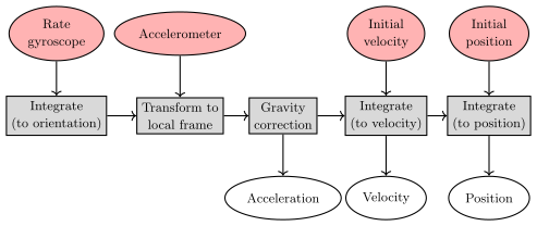
Figure 5.1: Inertial measurement unit (IMU) block diagram.

One of the fundamental issues with IMUs is the phenomenon called drift, which describes the slow accumulation of errors over time. Drift in any one component will also affect the downstream components. For example, drift in the gyroscope leads to errors in the estimation of the vehicle orientation relative to gravity, which results in incorrect cancellation of the gravity vector. Additionally, errors in acceleration measurements will cause the integrated velocity to drift in time, which will in turn also cause position estimate drift. We can account for drift by using periodic references to some external measurement, such as GNSS position measurements, cameras, or other sensors.

Heading sensors.

Heading sensors determine the robot’s orientation in space and can be proprioceptive (gyroscopes) or exteroceptive (compasses). Compasses measure the Earth’s magnetic field to provide an estimate of direction. Digital compasses using the Hall effect are inexpensive but often suffer from poor resolution and accuracy, while flux-gate compasses have improved resolution and accuracy but are more expensive. Both types are vulnerable to magnetic field disturbances, making them less suitable for indoor applications. Gyroscopes preserve their orientation with respect to a fixed inertial reference frame and can be mechanical or optical. While high-quality gyroscopes can achieve excellent accuracy (angular drift of about 0.1 degrees in 6 hours), they are expensive and still suffer from drift over time.

5.4.2 Exteroceptive Sensors

Active ranging.

Active ranging sensors provide direct distance measurements to objects in the vicinity of the sensor. These sensors are important in robotics for localization and environment reconstruction. There are two main types of active ranging sensors: time-of-flight active ranging sensors and geometric active ranging sensors^†^†margin: Examples of time-of-flight sensors include ultrasonic, laser rangefinder, and time-of-flight cameras, and examples of geometric sensors include optical triangulation and structured light sensors. .

1.

Time-of-flight Active Ranging: Time-of-flight active ranging sensors make use of the propagation speed of sounds or electromagnetic waves. In particular, the travel distance is given by:

$d=\frac{ct}{2},$

where $d$ is the distance to the target, $c$ is the speed of wave propagation, and $t$ is the measured round-trip time of flight. Note that the time of flight is significantly smaller when using electromagnetic signals, on the order of nanoseconds for distances on the order of meters, which can make these types of sensors more challenging to develop in an affordable and robust way. The quality of time-of-flight range sensors depends on several factors including uncertainties in determining the exact time of arrival of the reflected signal, inaccuracies in the time of flight measurement, the dispersal cone of the transmitted beam^†^†margin: Mainly with ultrasonic range sensors. , interaction with the target^†^†margin: For example, surface absorption, specular reflections. , and the speed of the mobile robot and dynamic targets.
2.

Geometric Active Ranging: Geometric active ranging sensors use geometric properties in the measurements to establish distance readings. Generally, these sensors project a known pattern of light and then we can use geometric properties to analyze the reflection and estimate range via triangulation. Optical triangulation sensors (1D) transmit a collimated beam toward the target and use a lens to collect reflected light and project it onto a position-sensitive device or linear camera. Structured light sensors (2D or 3D) project a known light pattern such as a point, line, or texture, onto the environment. The reflection is captured by a receiver and then, together with known geometric values, we can estimate range via triangulation.

Beacons.

Beacons are signaling devices with precisely known positions^†^†margin: Stars and lighthouses are classic examples. that enable position determination through relative measurements. The GNSS positioning system is an advanced example of beacons that works by processing synchronized signals from at least four satellites to estimate three position coordinates and a clock correction variable. Indoor positioning systems often use camera-based motion capture or ultra-wideband beacons for similar functionality in GPS-denied environments.

Vision sensors.

Vision sensors have become crucial for perception in robotics due to their ability to capture an enormous amount of information about the environment^†^†margin: The human eye provides millions of bits of information per second. . Unlike the sensors discussed above which provide specific measurements like distance or orientation, cameras capture rich visual data that can be processed to extract various types of information including object detection, depth estimation, motion tracking, and scene understanding. The main challenges associated with vision-based sensing are related to processing digital images to extract salient information like object depth, motion and object detection, color tracking, feature detection, scene recognition, and more. We generally refer to the analysis and processing of images as computer vision and image processing. The next chapter will explore camera models and calibration in detail, followed by techniques for extracting 3D information from visual data.

5.5 Summary

This chapter introduced the fundamental concepts of robot sensors, including their classifications, performance metrics, and common types used in mobile robotics. Understanding sensor characteristics—including their limitations and error sources—is essential for effective robot perception. While we’ve surveyed various sensor types, the remainder of this part will focus specifically on vision-based sensing, beginning with camera models and calibration in the next chapter. Later chapters will introduce how these sensors can be used to extract useful information about the environment, such as object detections.

To learn more.

To dive deeper into robot sensors and perception, Introduction to Autonomous Mobile Robots by Siegwart et al. (2011)¹1. Siegwart, R., Nourbakhsh, I. R., Scaramuzza, D. Introduction to Autonomous Mobile Robots. MIT Press, 2011. provides a comprehensive overview of various sensor types and their applications in robotics. Additionally, readers interested in robotic sensor details are encouraged to read Dudek and Jenkin (2008)²2. Dudek, G., Jenkin, M. “Inertial Sensors, GPS, and Odometry.” In Springer Handbook of Robotics, 477–490. Springer, 2008..