Classical Methods for Perception · Principles of Robot Autonomy

The previous chapters focused on using camera models to identify the relationship between points in a 3D scene and their projections onto the camera image, as well as how to leverage those models to reconstruct 3D scene structure from images. In this chapter, we introduce methods for extracting various types of information from images through both low-level image processing and higher-level feature extraction techniques.

We begin with image processing fundamentals, including filtering, feature detection, and description in Section 8.1. We then discuss geometric feature extraction methods in Section 8.2 for identifying structure in sensor data. Finally, in Section 8.3, we cover feature-based object detection approaches and discuss how classical perception methods remain relevant in modern robotics applications.

8.1 Image Processing Fundamentals

At its core, image processing is a form of signal processing where the input signal is an image, such as a photo or a video, and the output is either an image or a set of parameters associated with the image. Extracting visual content from raw images is important for mobile robots to be able to intelligently interpret their surroundings^†^†margin: Information extracted through image processing can have a significant impact on a robot’s ability to perform fundamental tasks including localization, mapping, and decision making. . While a large number of image processing techniques exist, in this chapter, we focus on some of the more fundamental methods that are relevant for robotics⁷7. Siegwart, R., Nourbakhsh, I. R., Scaramuzza, D. Introduction to Autonomous Mobile Robots. MIT Press, 2011..

8.1.1 Image Filtering

Image filtering is one of the principal tasks in image processing. The term filter comes from frequency domain signal processing and refers to the process of accepting or rejecting certain frequency components of a signal^†^†margin: For example, eliminating high-frequency noise is a classic filtering problem. . Perhaps the most common type of image filtering is spatial filtering. The basic principle of spatial filtering is that a particular pixel is modified in the filtered image based on the pixels in the immediate spatial neighborhood, as we show in Figure 8.1.

Mathematically, we describe an image as a function, $I(x,y)$ , that maps a pixel at coordinate $(x,y)$ in the domain $[a,b]\times[c,d]$ to either a scalar for grayscale images or a three-dimensional vector corresponding to red, green, and blue values for color images. A spatial filter for an image, $I(x,y)$ , consists of a neighborhood of pixels around a particular point, $(x,y)$ , under examination, which we denote as $S_{xy}$ ^†^†margin: This region is typically rectangular. , and a predefined operation, $F$ , that is performed on the image pixels encompassed by the neighborhood $S_{xy}$ . We define a new image, $I^{\prime}(x,y)$ , by applying the spatial filter operation $F$ to all pixels, $(x,y)$ , in the original image, $I$ .

Refer to caption — Figure 8.1: Illustration of the concept of spatial filtering. The spatial filter operates on a neighborhood, $S_{xy}$ , of each point in the original image to produce a new pixel in the filtered image.

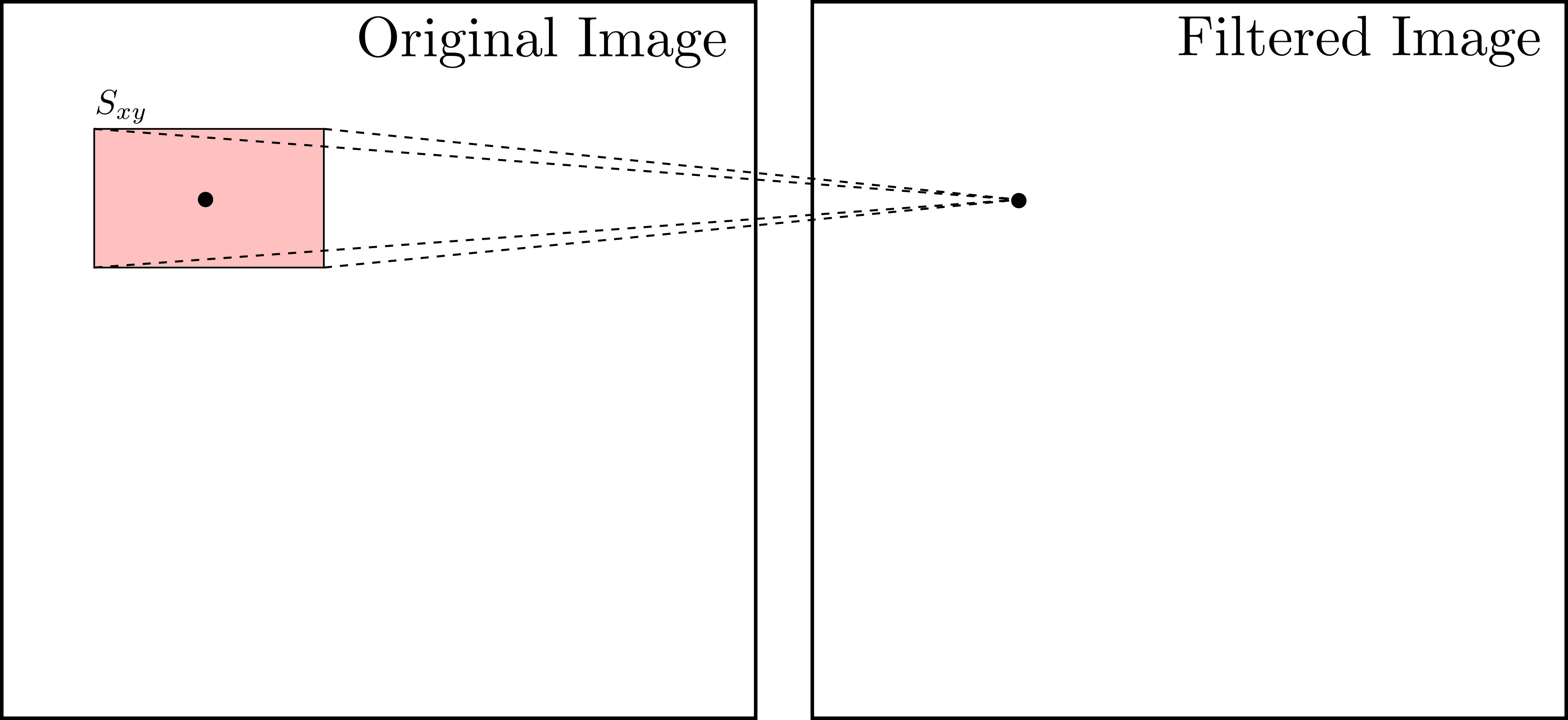
In general, filters can leverage linear or nonlinear operations, but many of the most fundamental filters are linear and we can express them mathematically as:

I^{\prime}(x,y)=F\circ I=\sum_{i=-N}^{N}\sum_{j=-M}^{M}F(i,j)I(x+i,y+j),

(8.1)

where $N$ and $M$ are integers that define the width and height of a rectangular neighborhood, $S_{xy}$ . Based on the size of this neighborhood, we say that this filter is of size $(2N+1)\times(2M+1)$ . We generally refer to the filter operation $F$ as a mask or kernel. Broadly speaking, we refer to filters expressed by Equation 8.1 as correlation filters.

Convolution filters are another class of linear filters that we commonly use. Convolution filters are similar to correlation filters, but use reverse image indices^†^†margin: In fact, correlation and convolution filters are identical when the filter mask is symmetric in both the horizontal and vertical directions. . In particular, we express convolution filters mathematically by:

I^{\prime}(x,y)=F\ast I=\sum_{i=-N}^{N}\sum_{j=-M}^{M}F(i,j)I(x-i,y-j).

(8.2)

Convolution filters are associative, meaning that for two different filter masks, $F$ and $G$ , it is true that $F*(G*I)=(F*G)*I$ . This associative property is useful for tasks such as smoothing an image before applying a differentiation filter. Suppose the mask $F$ implements a derivative filter and $G$ implements a smoothing filter, then sequentially applying these filters would result in $F*(G*I)$ . However, because of the associative property, we can convolve the masks together first such that only the single filter $(F*G)*I$ needs to be applied to the image.

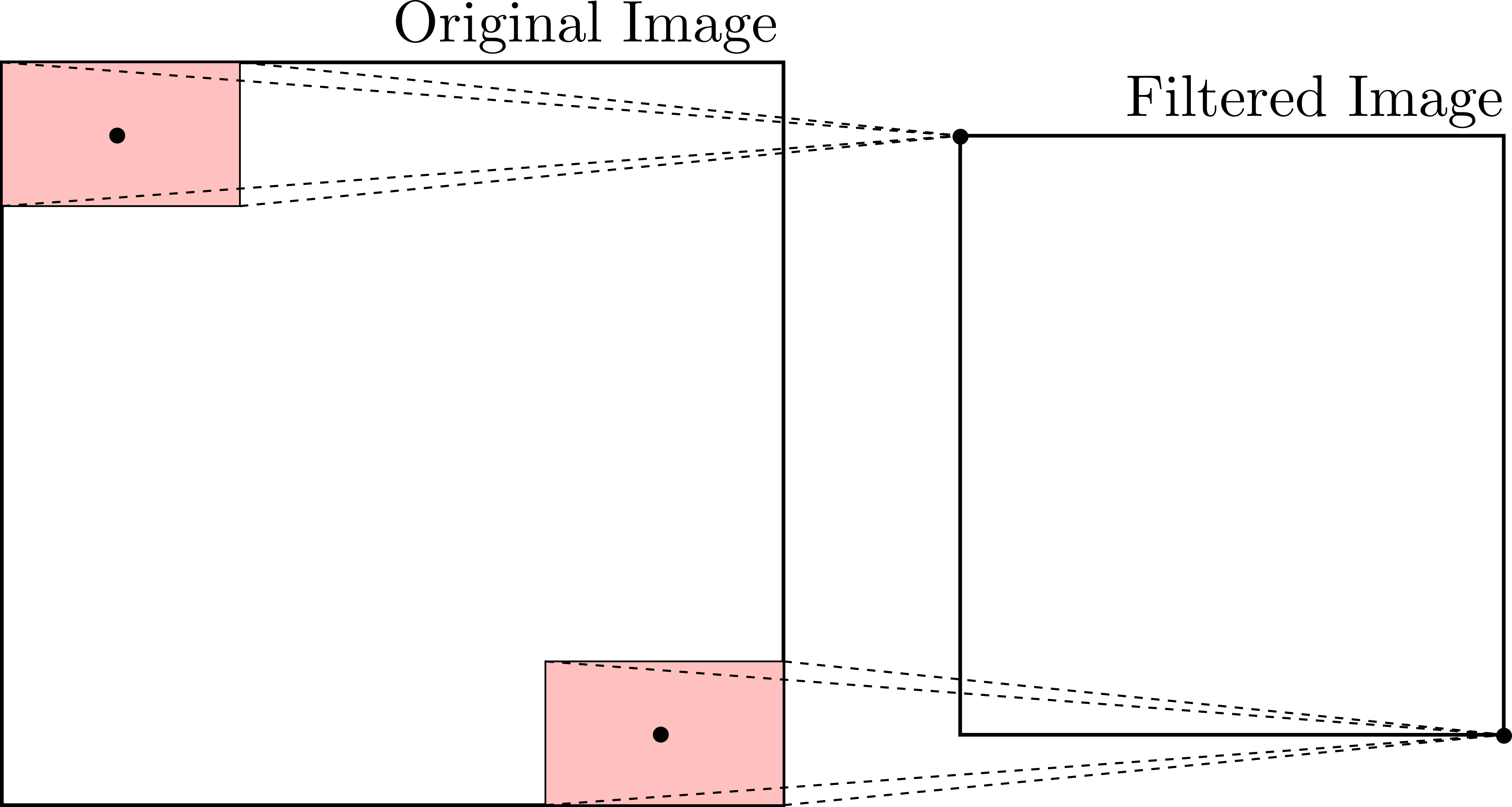
Note that in both correlation and convolution filters, the boundaries of the image need some special care because of the width and height of the mask. For example, in Figure 8.2 we show how the filtered image is smaller than the original due to the width and height of the mask. Some possible options to handle this include padding the image, cropping it, extending it, or wrapping it. However, as images are generally quite large relative to the mask size, the exact approach likely won’t vary the final result significantly.

Example 8.1.1 (Practical tricks for image filtering).

When implementing correlation and convolution filters, we can leverage special tricks to simplify the process. In this example, we introduce two simplification tricks: a change in indexing and zero-padding.

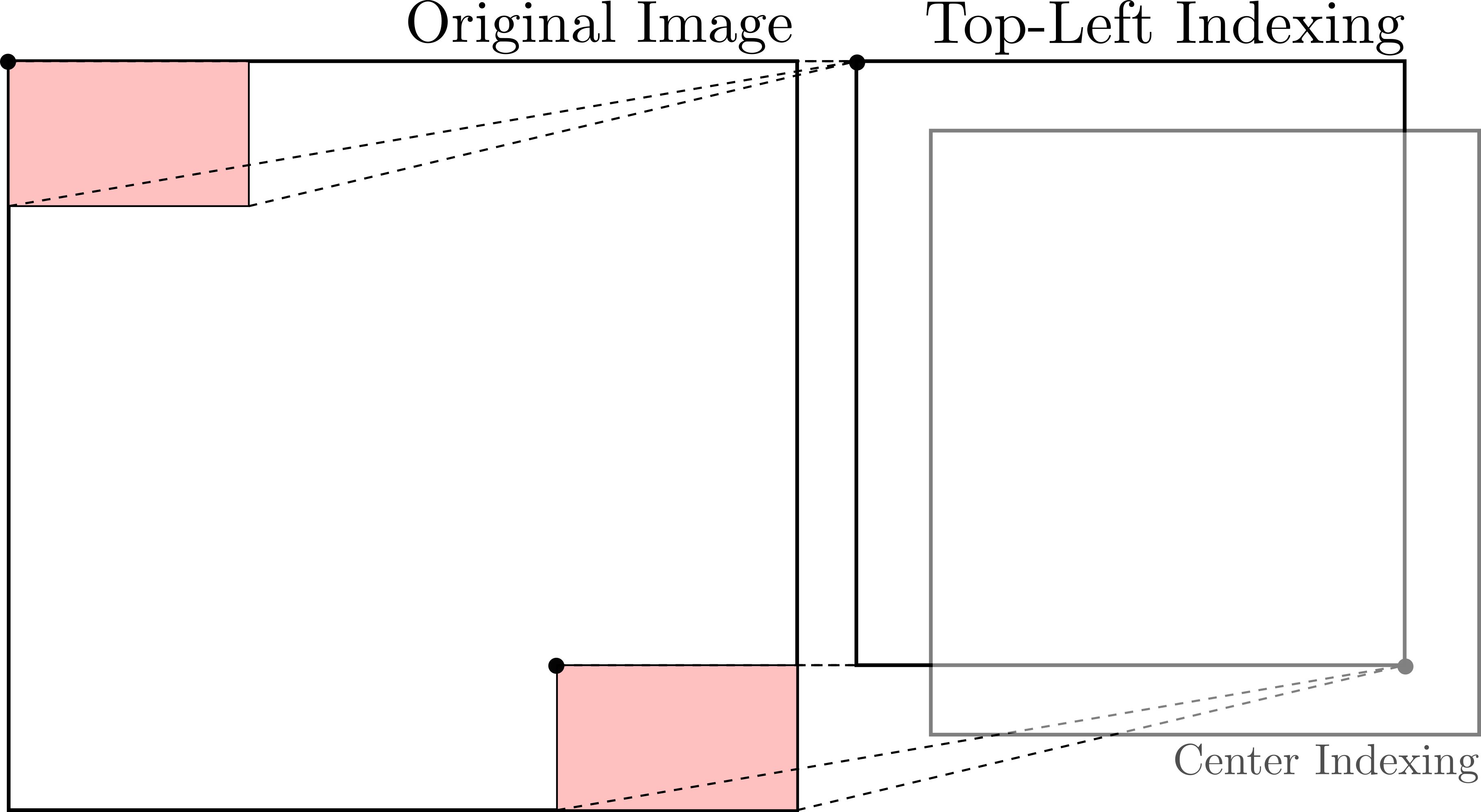
First, to accommodate varying sizes of filters, including even and odd sized filters, we can change the indexing such that the coordinate of interest is associated with the top-left element in the window rather than the center. For a correlation filter, this would correspond to:

I^{\prime}(x,y)=F\circ I=\sum_{i=0}^{K-1}\sum_{j=0}^{L-1}F(i,j)I(x+i,y+j),

(8.3)

where $K$ and $L$ are integers that define the width and height of the filter, and the pixel $(x,y)$ is at row $x$ and column $y$ . Note that this formulation results in an output image, $I^{\prime}$ , that is shifted up and to the left. To see this shift, consider the top-left pixel at $x=0$ and $y=0$ in the new image, $I^{\prime}$ . We generate this new pixel value by applying the filter, $F$ , over the pixels in the original image at rows $\{0,\dots,K-1\}$ and columns $\{0,\dots,L-1\}$ , which is not centered at $(0,0)$ in the original image, $I$ . In practice, this shifting is not an issue as long as we always index with respect to the top-left corner. We show an example of top-left indexing in Figure 8.3.

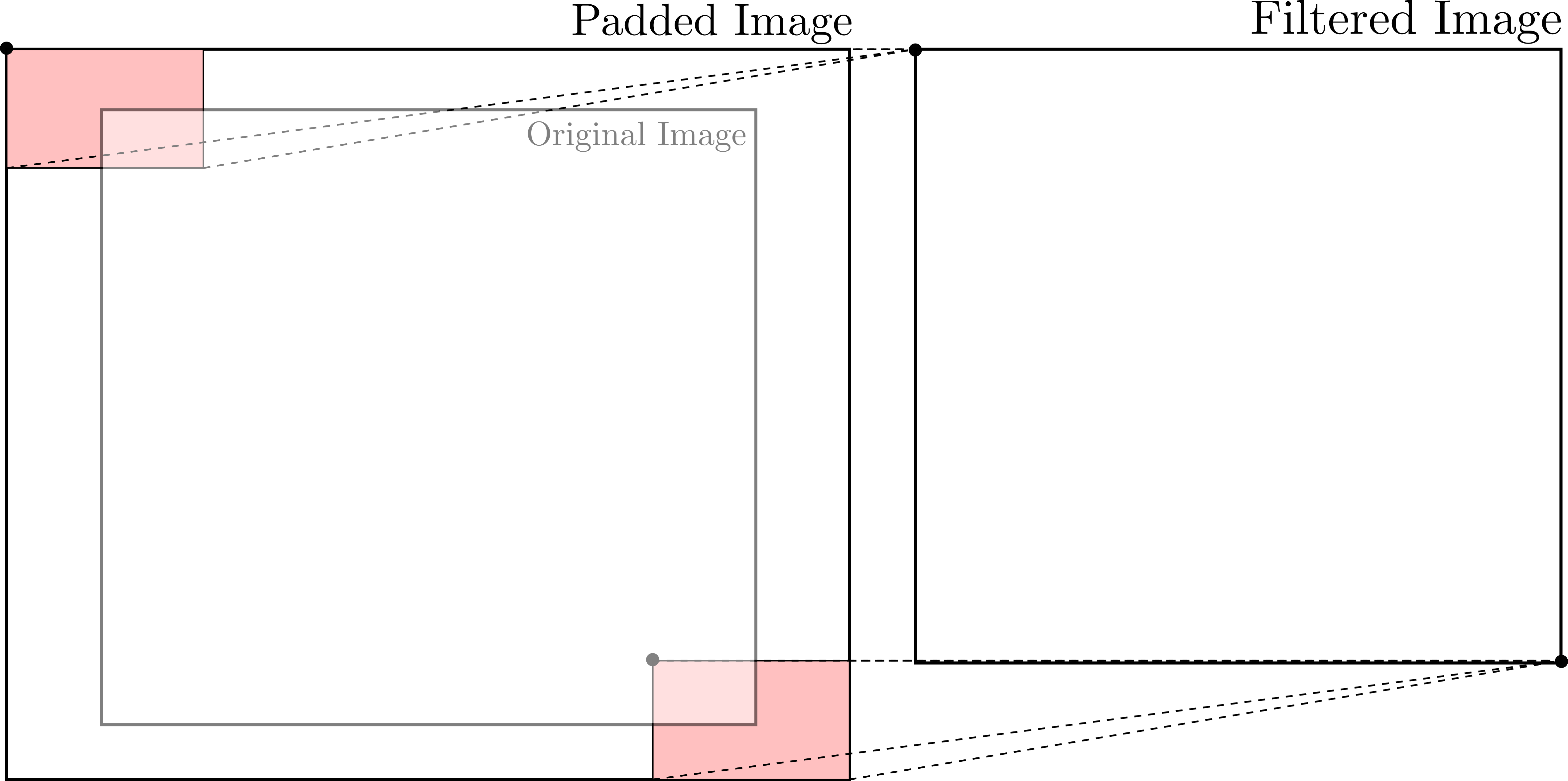
Zero-padding^†^†margin: Also commonly referred to as same padding. is another simple trick that we can use to ensure that the output filtered image, $I^{\prime}$ , has the same dimension as the input image, $I$ . In this approach, we pad the left and right boundaries of the image by $\lfloor K/2\rfloor$ columns of zeros, and pad the top and bottom boundaries by $\lfloor L/2\rfloor$ rows of zeros, where $\lfloor\cdot\rfloor$ denotes the floor operation. For example, the image:

I=\begin{bmatrix}1&2&3\\ 4&5&6\\ 7&8&9\\ \end{bmatrix},

becomes:

I_{\text{padded}}=\begin{bmatrix}0&0&0&0&0\\ 0&1&2&3&0\\ 0&4&5&6&0\\ 0&7&8&9&0\\ 0&0&0&0&0\\ \end{bmatrix},

for filters $F\in\mathbb{R}^{3\times 3}$ , $F\in\mathbb{R}^{2\times 2}$ , $F\in\mathbb{R}^{2\times 3}$ and $F\in\mathbb{R}^{3\times 2}$ . When using this padding rule with a correlation filter from Equation 8.3 and a filter, $F$ , with $K=2,3$ and $L=2,3$ , we can define the new image, $I^{\prime}$ , for values $x\in\{1,2,3\}$ and $y\in\{1,2,3\}$ , resulting in $I^{\prime}$ being the same dimension as the original image, $I$ . We show an example use of padding combined with top-left indexing graphically in Figure 8.4.

Moving average filter.

The moving average filter returns the average of the pixels in the mask, which achieves a smoothing effect^†^†margin: Smoothing removes sharp features in the image. . For example, we can define a moving average filter with a normalized^†^†margin: The normalization is used to maintain the overall brightness of the image. $3\times 3$ mask with $F$ from Equation 8.1 defined as:

F=\frac{1}{9}\begin{bmatrix}1&1&1\\ 1&1&1\\ 1&1&1\\ \end{bmatrix}.

Due to the symmetry of the mask, the correlation filter from Equation 8.1 and convolution filter from Equation 8.2 will be identical.

Gaussian smoothing filter.

Gaussian smoothing filters are similar to the moving average filter, but instead of weighting all of the pixels evenly they are weighted by the Gaussian function:

G_{\sigma}(x,y)=\frac{1}{2\pi\sigma^{2}}\exp\bigg{(}-\frac{x^{2}+y^{2}}{2% \sigma^{2}}\bigg{)}.

We use this function to obtain the mask operation, $F$ , by sampling the function about the center pixel. For example, for the center pixel with $i=j=0$ in Equation 8.1, we sample $G_{\sigma}(0,0)$ . For a normalized $3\times 3$ mask with $\sigma=0.85$ , this filter is approximately defined by:

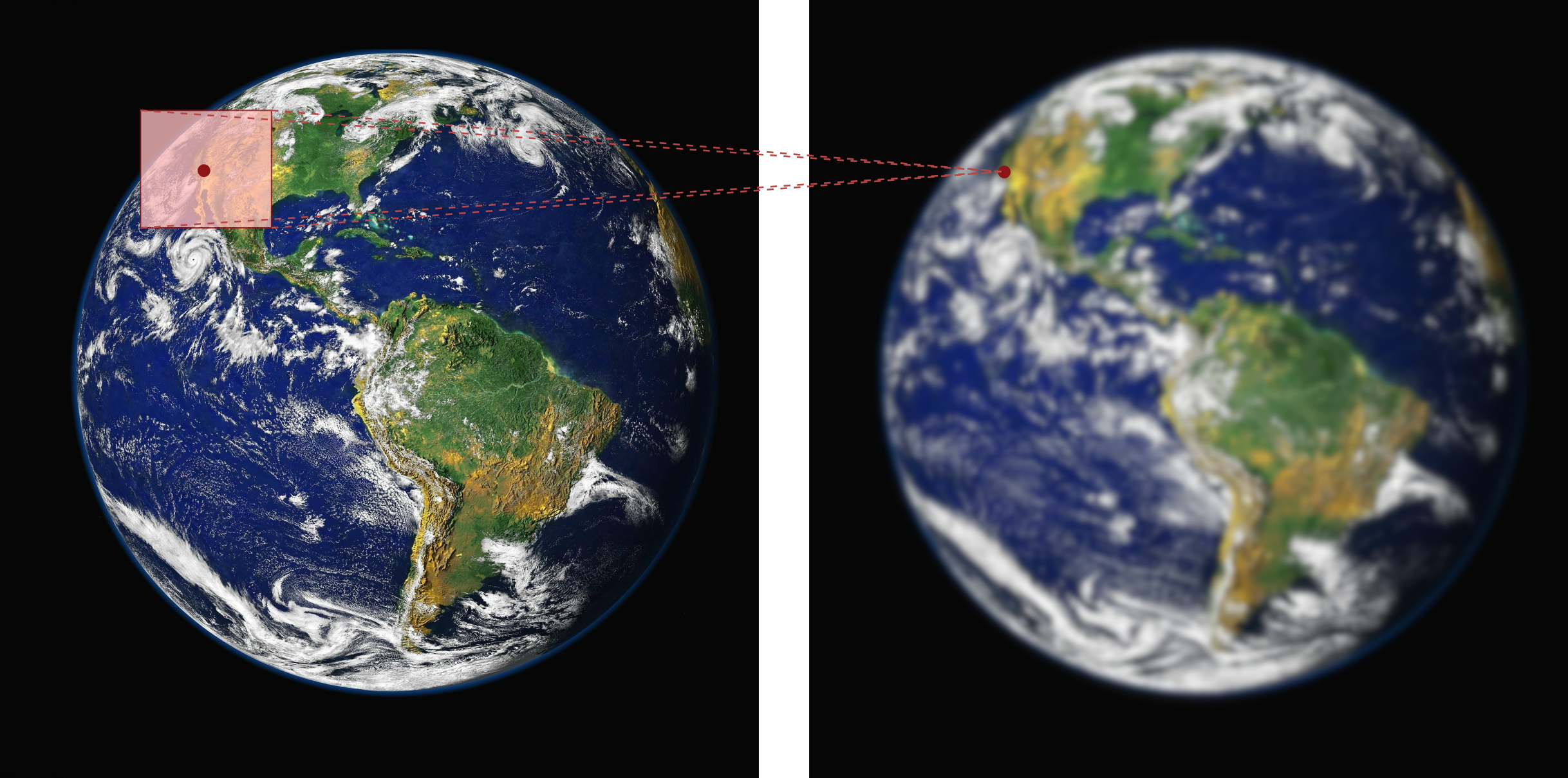
F=\frac{1}{16}\begin{bmatrix}1&2&1\\ 2&4&2\\ 1&2&1\end{bmatrix}.

Like the moving average filter, this filter mask is symmetric and therefore yields identical results with respect to the correlation or convolution filters. The advantage of the Gaussian filter is that it provides more weight to the neighboring pixels that are closer. We show an example of this filter in Figure 8.5.

Separable masks.

We call a mask separable if it can be broken down into the convolution of two kernels, $F=F_{1}\ast F_{2}$ . If a mask is separable into smaller masks, then it is often cheaper to apply $F_{1}$ followed by $F_{2}$ , rather than by $F$ directly. One special case of this is when we can represent the mask as an outer product of two vectors, meaning it is equivalent to the 2D convolution of those two vectors. If a separable mask has shape $M\times M$ and the input image has size $w\times h$ , then the computational complexity of directly performing the convolution is $O(M^{2}wh)$ . By separating the masks, the computational cost is $O(2Mwh)$ , which is linear in $M$ rather than quadratic. As an example, consider the moving average filter mask from before:

F=\frac{1}{9}\begin{bmatrix}1&1&1\\ 1&1&1\\ 1&1&1\end{bmatrix}=\frac{1}{9}\begin{bmatrix}1\\ 1\\ 1\end{bmatrix}\begin{bmatrix}1&1&1\\ \end{bmatrix}.

As another example, we note that the Gaussian smoothing filter mask is also separable. To see why this is, note that we can decompose the Gaussian weighting function as:

\begin{split}G_{\sigma}(x,y)&=\frac{1}{2\pi\sigma^{2}}\exp\bigg{(}-\frac{x^{2}% +y^{2}}{2\sigma^{2}}\bigg{)}\\ &=\frac{1}{\sqrt{2\pi}\sigma}\exp\bigg{(}-\frac{x^{2}}{2\sigma^{2}}\bigg{)}% \frac{1}{\sqrt{2\pi}\sigma}\exp\bigg{(}-\frac{y^{2}}{2\sigma^{2}}\bigg{)}\\ &=g_{\sigma}(x)\cdot g_{\sigma}(y).\end{split}

Image differentiation filters.

We can identify some image features, such as edges, by looking at the spatial derivatives in the pixel intensity values in both the vertical and horizontal directions. Since we represent images as functions defined over a discrete domain, the traditional method for differentiating continuous functions is not applicable. Instead, we can compute differences between pixels using techniques like the central difference method:

\begin{split}\frac{\partial I}{\partial x}&=\frac{I(x+1,y)-I(x-1,y)}{2},\\ \frac{\partial I}{\partial y}&=\frac{I(x,y+1)-I(x,y-1)}{2}.\end{split}

(8.4)

where $\partial I/\partial x$ is the derivative in the horizontal direction and $\partial I/\partial y$ is the derivative in the vertical direction. We can also define the derivatives using just one side instead of a central difference, for example $\frac{\partial I}{\partial x}=I(x+1,y)-I(x,y)$ .

We can also differentiate an image using convolution filters. In particular, one common approach is to use a convolution filter of the form Equation 8.2 defined with a mask, $F$ , called a Sobel mask^†^†margin: Also referred to as simply a Sobel operator. . We denote this mask as $S_{x}$ for the $x$ direction and $S_{y}$ for the $y$ direction:

S_{x}=\begin{bmatrix}1&0&-1\\ 2&0&-2\\ 1&0&-1\end{bmatrix},\quad S_{y}=\begin{bmatrix}1&2&1\\ 0&0&0\\ -1&-2&-1\end{bmatrix}.

(8.5)

Sobel masks are similar to the central difference method but use more neighboring pixels when calculating the derivative^†^†margin: Specifically, they also consider the rows above and below to compute the difference. . Note that Sobel masks are separable.

Similarity measures.

We can also use filtering to find similar features in different images, which can be useful for solving the correspondence problem in stereo vision or structure-from-motion techniques. In particular, we can compute the similarity between the pixel $(x,y)$ in image $I_{1}$ and pixel $(x^{\prime},y^{\prime})$ in image $I_{2}$ by:

\begin{split}SAD&=\sum_{i=-N}^{N}\sum_{j=-M}^{M}\lvert I_{1}(x+i,y+j)-I_{2}(x^% {\prime}+i,y^{\prime}+j)\rvert,\\ SSD&=\sum_{i=-N}^{N}\sum_{j=-M}^{M}[I_{1}(x+i,y+j)-I_{2}(x^{\prime}+i,y^{% \prime}+j)]^{2},\end{split}

(8.6)

where SAD is an acronym for sum of absolute differences, SSD is an acronym for sum of squared differences, and $N$ and $M$ define the size of the window around the pixels that we consider.

8.1.2 Image Feature Detection

A local feature^†^†margin: Also sometimes referred to as interest points, interest regions, or keypoints. in an image is a pattern that differs from its immediate neighborhood in terms of intensity, color, or texture. We can generally categorize local features in several ways, for example by whether or not they provide semantic content. For example, features that may provide semantic content include edges or other geometric shapes, such as lanes of a road or blobs corresponding to blood cells in medical images. Features that do not provide semantic content may also be useful, for example in feature tracking, camera calibration, 3D reconstruction, image mosaicing, and panorama stitching. In these cases, it may be more important that the feature be able to be located accurately and robustly over time. A third category of features are those that may not have semantic interpretations individually, but may have meaning as a collection. For instance, we could recognize a scene by counting the number of feature matches between the observed scene and a query image. In this case, only the number of matches is relevant and not the location or type of feature. Applications where these types of features are important include texture analysis, scene classification, video mining, and image retrieval.

We discuss several feature detection strategies below. While many strategies exist for different types of features, our focus will be on two common features that are often useful in robotics: edges and corners.

Edge detection.

An edge in an image is a region where there is a significant change in intensity values along one direction, and negligible change along the orthogonal direction. In one dimension an edge corresponds to a point where there is a sharp change in intensity, which mathematically can be thought of as a point of a function having a large first derivative and a small second derivative. Many edge detectors rely on this concept by differentiating images and looking for spikes in the derivative. We can evaluate an edge detector based on several criteria for robustness and performance, including accuracy, localization, and single response. Good accuracy implies few false positives or negatives^†^†margin: In this case, a false positive is a detection of an edge that isn’t real, and a false negative is a missed edge. , good localization implies that the detected edge should be exactly where the true edge is in the image, and a single response implies that only one edge is detected for each real edge. Noise and discretization effects can make edge detection challenging in practice.

Most edge detection methods rely on two key steps: smoothing and differentiation. We perform differentiation in both the vertical and horizontal directions to find locations in the image with high intensity gradients. However, differentiation alone is vulnerable to false positives due to image noise, which is why many algorithms will first smooth the image.

Example 8.1.2 (Edge detection in 1D).

In Figure 8.6, we show an example of how noise can corrupt image differentiation.

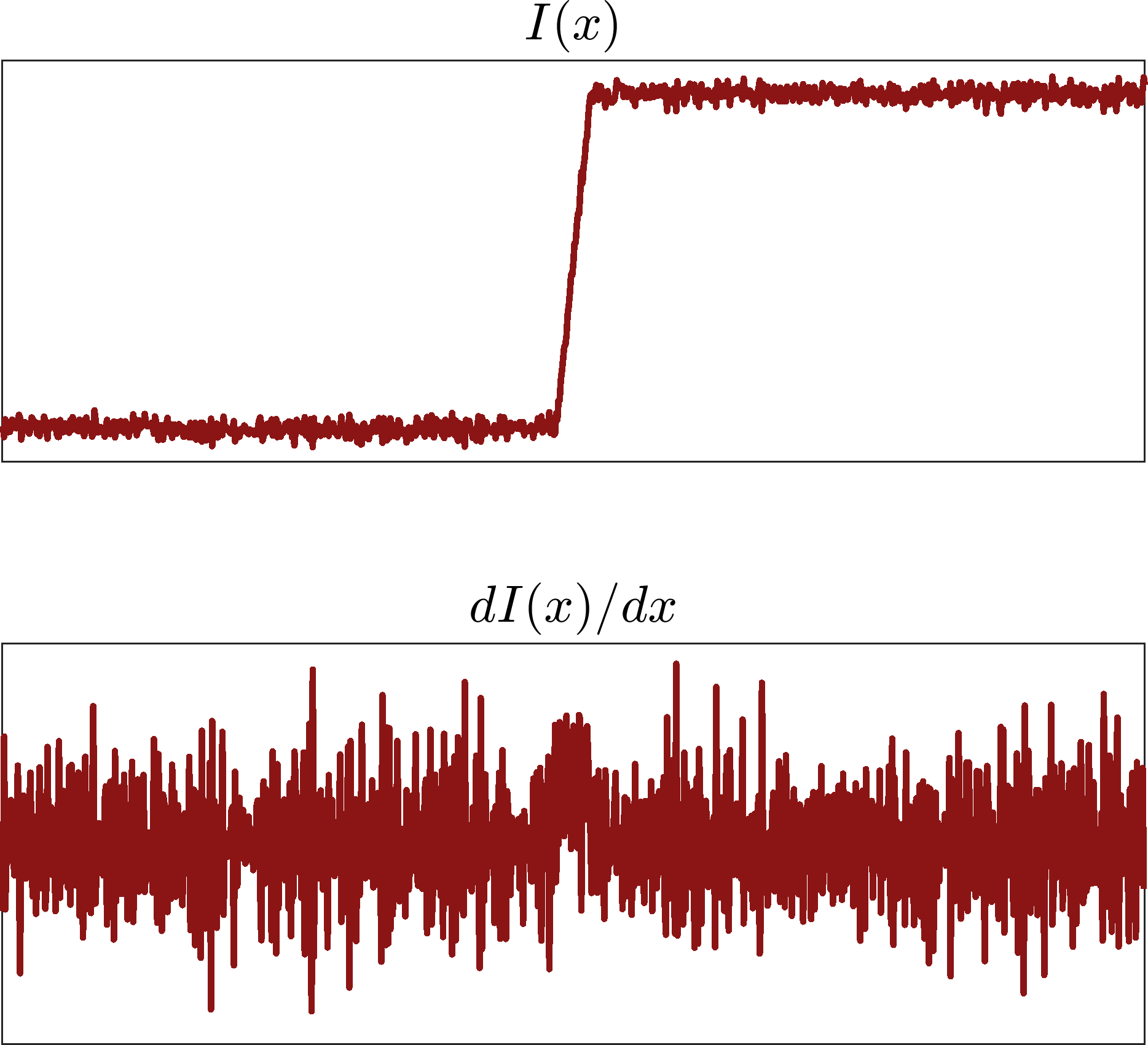
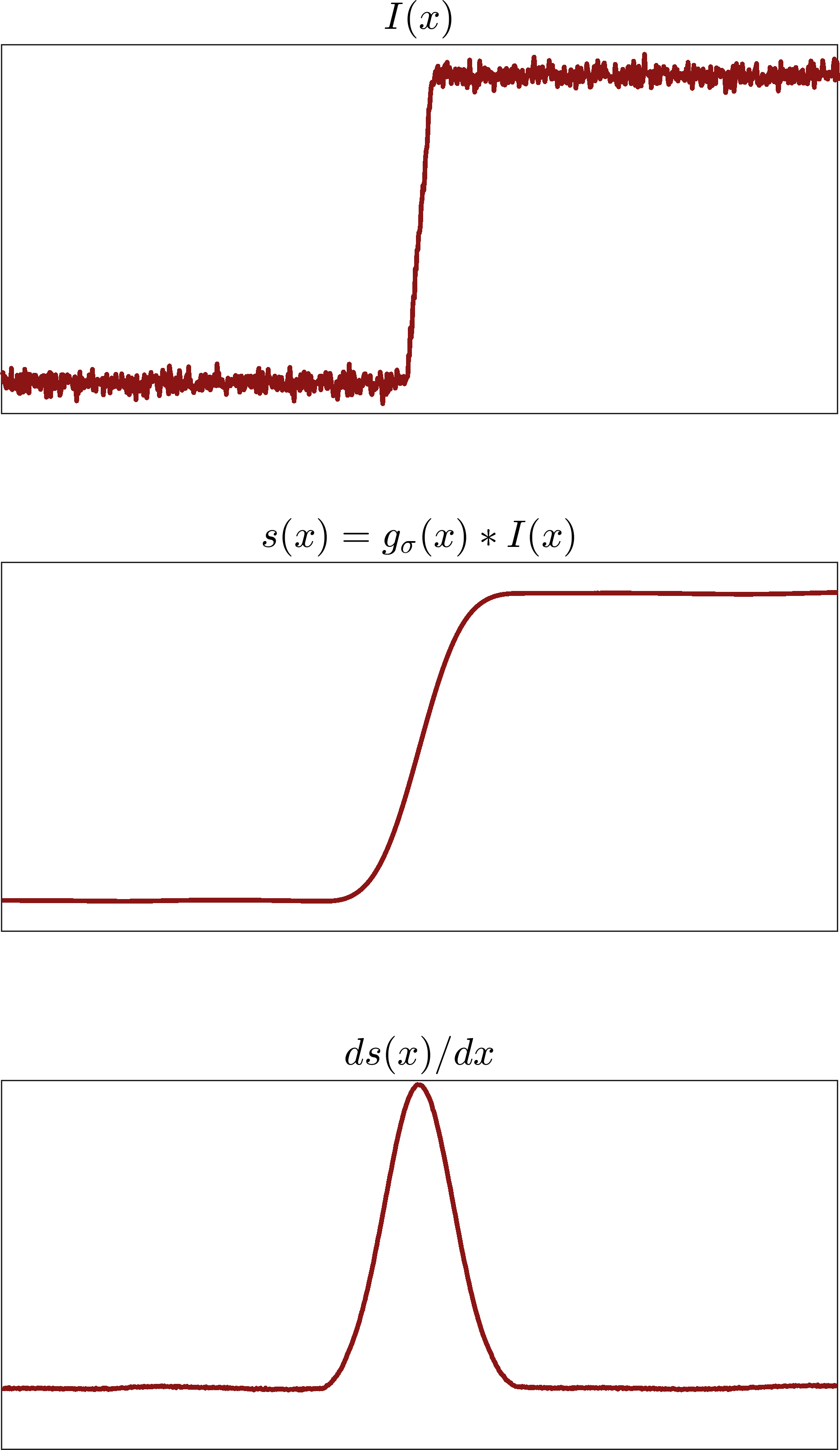
Notice that in this case it is impossible to identify the jump in the signal due to the noise levels. Smoothing filters, such as the Gaussian smoothing filter discussed earlier, can help remedy this problem. In particular, suppose the original signal in Figure 8.6 is defined by $I(x)$ . We can compute a smoothed version by applying a smoothing convolution filter:

s(x)=g_{\sigma}(x)\ast I(x),

where $g_{\sigma}(x)$ represents a Gaussian smoothing filter, and then by applying the differentiation filter:

s^{\prime}(x)=\frac{d}{dx}\ast s(x).

We show this process in Figure 8.7.

Note that since these filters are convolutions, we can leverage the associativity property to combine them into a single filter:

s^{\prime}=(\frac{d}{dx}*g_{\sigma})*I.

Example 8.1.3 (Edge detection in 2D).

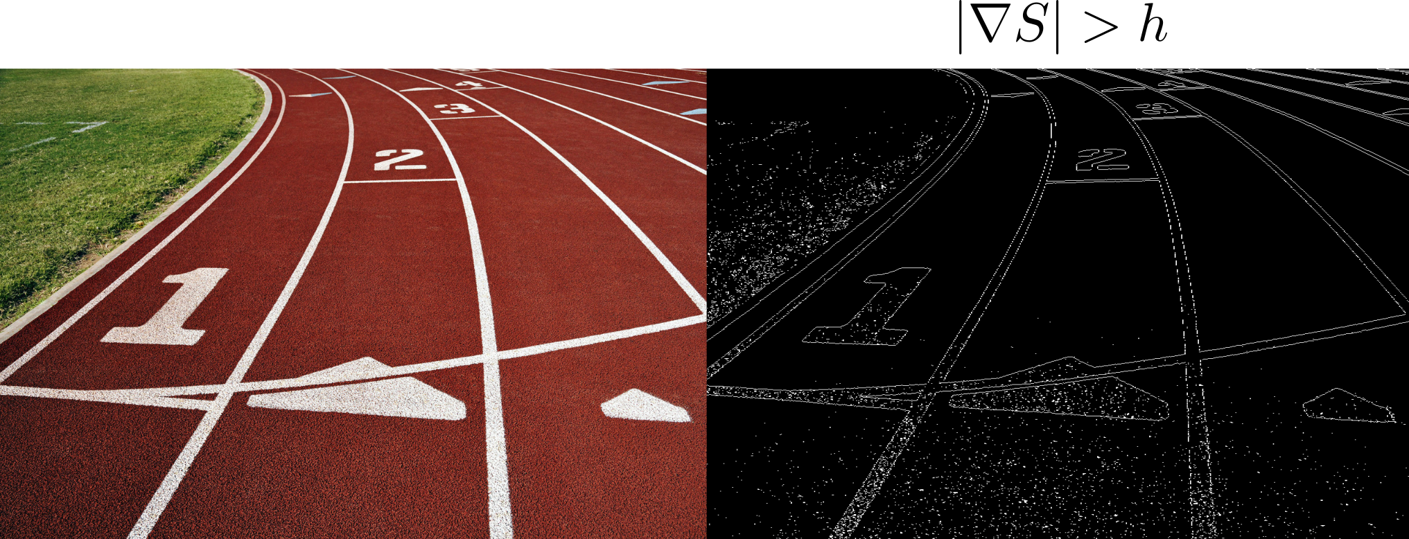
Edge detection in a two-dimensional image is quite similar to the example previously discussed for one dimension. Let the smoothing filter be the Gaussian smoothing filter from before, and consider a differentiation filter such as the Sobel filter. We can write the gradient of the smoothed image in both the $x$ and $y$ directions as:

\nabla S=\begin{bmatrix}\frac{\partial}{\partial x}*G_{\sigma}*I\\ \frac{\partial}{\partial y}*G_{\sigma}*I\end{bmatrix}=\begin{bmatrix}G_{\sigma% ,x}*I\\ G_{\sigma,y}*I\end{bmatrix}=\begin{bmatrix}S_{x}\\ S_{y}\end{bmatrix},

where $I$ is the original image and we use the associativity property of the smoothing and differentiation convolution filters to define the combined filters $G_{\sigma,x}$ and $G_{\sigma,y}$ . We can then compute the magnitude of the gradient by:

\lvert\nabla S\rvert=\sqrt{S_{x}^{2}+S_{y}^{2}},

which we can use to compare against a predefined threshold value for edge detection. To guarantee that we define thin edges, it is also possible to filter out points with gradient magnitude above the threshold that are not local maxima. We show an example of this process in Figure 8.8.

Corner detection.

A corner in an image is defined as an intersection of two or more edges, and also sometimes as a point where there is a large intensity variation in every direction. Important properties of corner detectors include repeatability and distinctiveness. The repeatability of a corner detector quantifies how well we can find the same features in multiple images even under geometric and photometric transformations. Distinctiveness refers to whether the information carried by the patch surrounding the feature is distinctive, which we can use to reliably produce correspondences. Both of these properties are particularly important in applications such as panorama stitching and 3D reconstruction.

We can generally think of corner detection in a similar way to edge detection, except that instead of looking for change along one direction there should be changes in all directions. One well-known corner detector is known as the Harris detector⁸8. Harris, C., Stephens, M. “A combined corner and edge detector.” In 4th Alvey Vision Conference, 1988., which has the useful property that the detection is invariant to rotations and linear intensity changes, such as geometric and photometric invariance. However, the Harris detector is not invariant to scale changes or geometric affine changes, which has led to the development of scale-invariant detectors such as the Harris-Laplacian detector or the scale-invariant feature transform (SIFT) detector.

8.1.3 Image Descriptors

Image descriptors describe features so that they can be compared across images, or used for object detection and matching. Similar to image detectors, it is desirable for image descriptors to be repeatable^†^†margin: For example, invariant with respect to pose, scale, and illumination. and distinct. Perhaps the simplest example of a descriptor is an $n\times m$ window of pixel intensities centered at the feature, which we can normalize to be illumination invariant. However, such a descriptor is not invariant to pose or scale and is not distinctive, and therefore is generally not useful in practice.

8.2 Geometric Feature Extraction

It is common in robotic localization and mapping to represent the environment using simple geometric primitives^†^†margin: Common geometric primitives include lines, circles, corners, and planes. that we can efficiently extract from sensor data. In this section, we present some techniques for line extraction from range data^†^†margin: Range data can generally come from a variety of sources, including laser rangefinders, radar, or even computer vision. . Lines are one of the most fundamental geometric primitives that we would want to extract from data, and techniques for extracting other primitives are conceptually similar.

There are two main challenges with extracting lines from range data. The first is segmentation, which is the task of identifying which data points belong to which line, and inherently also identifying how many lines there are. The second is fitting, which is the task of estimating the parameters that define a line given a set of points. For simplicity, in this chapter, we consider line extraction problems based on two-dimensional range data.

8.2.1 Line Segmentation

The line segmentation problem is to determine how many lines exist in a given set of data and which data points correspond to each line. We will discuss three popular algorithms for line segmentation: the split-and-merge algorithm, the random sample consensus (RANSAC) algorithm, and the Hough-transform algorithm.

Split-and-merge.

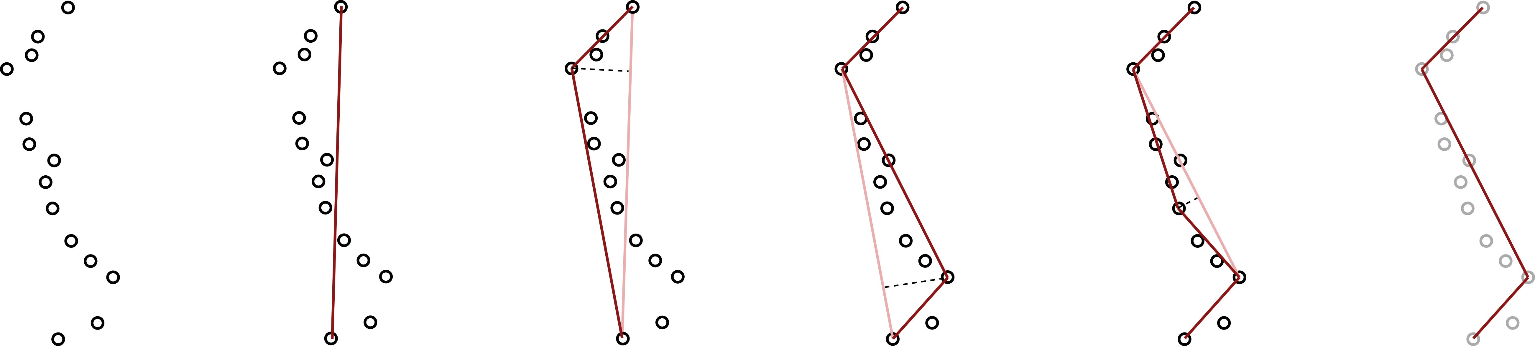
The split-and-merge algorithm is a popular line extraction algorithm that is fast but not very robust to outliers. The split-and-merge algorithm repeatedly fits lines to sets of points and then splits the set of points into two sets if any point lies more than a specified distance, $d$ , from the line. By repeating this process until no more splits occur, we are guaranteed that all points will lie less than the distance, $d$ , to a line. After this splitting process is complete, a second step merges any of the newly formed lines that are collinear. We present this algorithm in more detail in Algorithm 1.

Data: Set,

S

, of

N

points, distance threshold,

d>0

Result: A list,

L

, of sets of points, each resembling a line

L\xleftarrow{}[S]

i\xleftarrow{}1

while $i\leq\text{length}(L)$ do

Fit a line

(\alpha,r)

to the set

L[i]

Detect the point

P\in L[i]

with maximum distance,

D

, to the line

(\alpha,r)

if $D<d$ then

i\xleftarrow{}i+1

else

Split

L[i]

P

into new sets,

S_{1}

and

S_{2}

L[i]\xleftarrow{}S_{1}

L[i+1]\xleftarrow{}S_{2}

Merge collinear sets in

L

Algorithm 1 Split-and-Merge

A popular variant of the split-and-merge algorithm is known as the iterative-end-point-fit algorithm. This algorithm is the split-and-merge algorithm in Algorithm 1 where the line is constructed by simply connecting the first and the last points of the set. We show this approach graphically in Figure 8.9.

Random sample consensus (RANSAC).

Random Sample Consensus (RANSAC)⁹9. Fischler, Martin A., Bolles, Robert C. “Random sample consensus: a paradigm for model fitting with applications to image analysis and automated cartography.” Commun. ACM 24(6), 381–395, 1981. is an algorithm to estimate the parameters of a model from a set of data that may contain outliers^†^†margin: This problem is sometimes referred to as robust model parameter estimation. . Outliers are data points that do not fit the model and may be the result of high noise in the data, incorrect measurements, or simply points which come from objects that are unrelated to the current model. For example, a laser scan of an indoor environment may contain distinct lines from the surrounding walls but also points from other static and dynamic objects such as chairs or humans. In this case, if the goal is to extract lines to represent the walls, then any data point corresponding to other objects would be an outlier. In general, we can apply RANSAC to many parameter estimation problems, and typical applications in robotics include line extraction from 2D range data, plane extraction from 3D point clouds, and structure-from-motion^†^†margin: Where the goal in structure-from-motion problems is to identify image correspondences which satisfy a rigid body transformation. . We focus on using RANSAC for line extraction from two-dimensional data below.

RANSAC is an iterative method and is non-deterministic^†^†margin: In other words, it is stochastic or random. Running the algorithm twice on the same inputs will not necessarily produce the same results. . Given a dataset, $S$ , of $N$ points, we start by randomly selecting a sample of two points from $S$ . Next, we construct a line from the two sampled points and compute the distance of all other points to this line. We then define the set of inliers, which is comprised of all points whose distance to the line is within a predefined threshold, $d$ . By repeating this process $k$ times, we generate $k$ inlier sets and their associated lines and return the inlier set with the most points. We detail this procedure in Algorithm 2 and illustrate the process in Figure 8.10.

Data: Set,

S

, of

N

points, distance threshold,

d

Result: Set with maximum number of inliers and corresponding line

while $i\leq k$ do

Randomly select two points from

S

Fit line,

l_{i}

, through the two points.

Compute distance of all other points to

l_{i}

Construct set of points,

\tilde{S}_{i}

, with distance less than

d

l_{i}

Store line,

l_{i}

, and set of points,

\tilde{S}_{i}

i\xleftarrow{}i+1

Choose set

\tilde{S}_{i}

with maximum number of points.

Algorithm 2 Random Sample Consensus (RANSAC) for Line Extraction

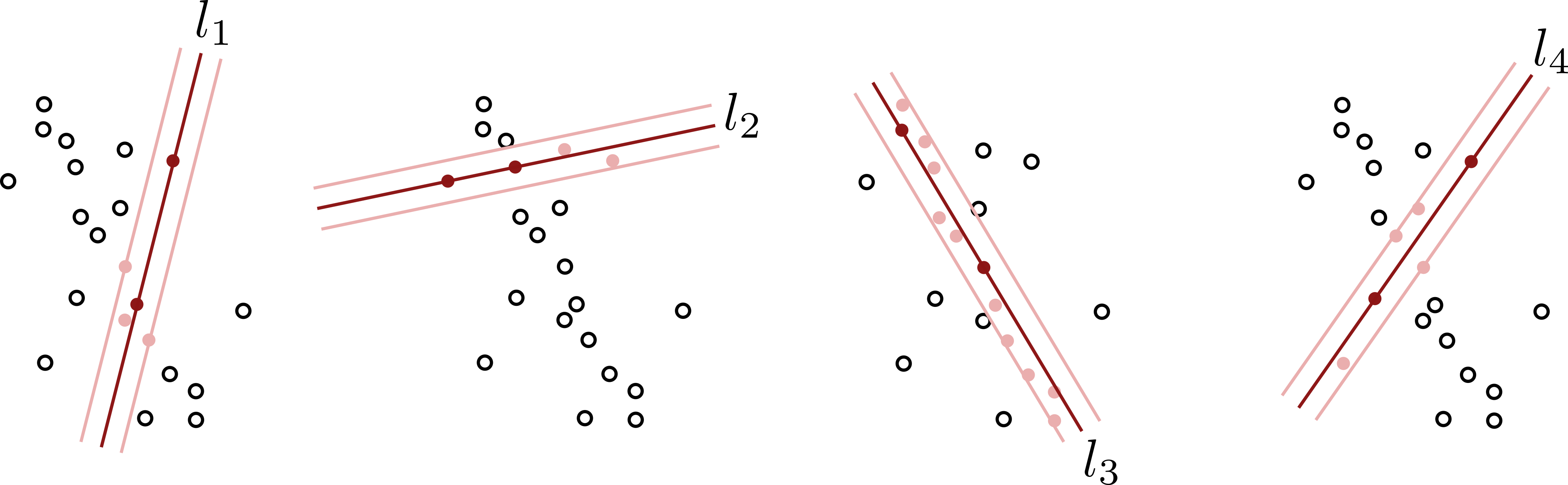
Due to the probabilistic nature of the algorithm, as the number of iterations, $k$ , increases the probability of finding a good solution increases. This approach is used over a brute force search of all possible combinations of two points since the total number of combinations is $N(N-1)/2$ , which can be extremely large. In fact, we can perform a simple statistical analysis of RANSAC. Let $p$ be the desired probability of finding a set of points free of outliers and let $w$ be the probability of selecting an inlier from the dataset, $S$ , of $N$ points, which we can express as:

w\coloneqq\frac{\text{\# inliers}}{N}.

Assuming we draw point samples independently from $S$ , the probability of drawing two inliers is $w^{2}$ , and $1-w^{2}$ is the probability that at least one is an outlier. Therefore, with $k$ iterations, the probability that RANSAC never selects two points that are both inliers is $(1-w^{2})^{k}$ . We can therefore find the minimum number of iterations, $\bar{k}$ , needed to find an outlier-free set with probability $p$ by solving:

1-p=(1-w^{2})^{k},

for $k$ . In other words, we can compute $\bar{k}$ as:

\bar{k}=\frac{\log(1-p)}{\log(1-w^{2})}.

While the value of $w$ may not be known exactly^†^†margin: There are advanced versions of RANSAC that can estimate $w$ in an adaptive online fashion. , we can still use this expression to get a good estimate of the number of iterations, $k$ , that we need for good results. It is important to note that this probabilistic approach often leads to a much smaller number of iterations than a brute force search through all combinations. We can attribute this to the fact that $\bar{k}$ is only a function of $w$ and not the total number of samples, $N$ , in the dataset.

Overall, the main advantage of RANSAC is that it is a generic extraction method and can be used with many types of features given a feature model. It is also simple to implement and is robust to data outliers. The main disadvantages are that the algorithm needs to run multiple times to extract multiple features, and there are no guarantees that the solutions will be optimal.

Hough transform.

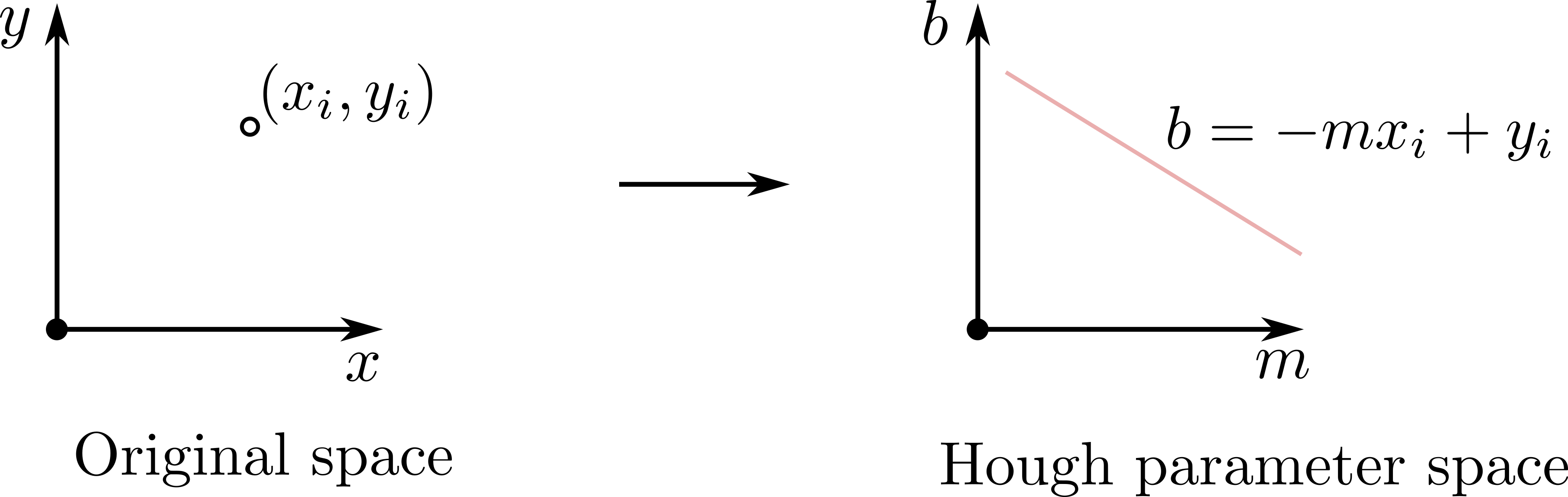
In the Hough transform algorithm, each point, $(x_{i},y_{i})$ , of the dataset, $S$ , votes for a set of possible line parameters, $(m,b)$ , where $m$ is the slope and $b$ is the intercept point. For any given point, $(x_{i},y_{i})$ , the candidate set of line parameters, $(m,b)$ , that could pass through this point must satisfy $y_{i}=mx_{i}+b$ , which we can also write as:

\quad b=-mx_{i}+y_{i}.

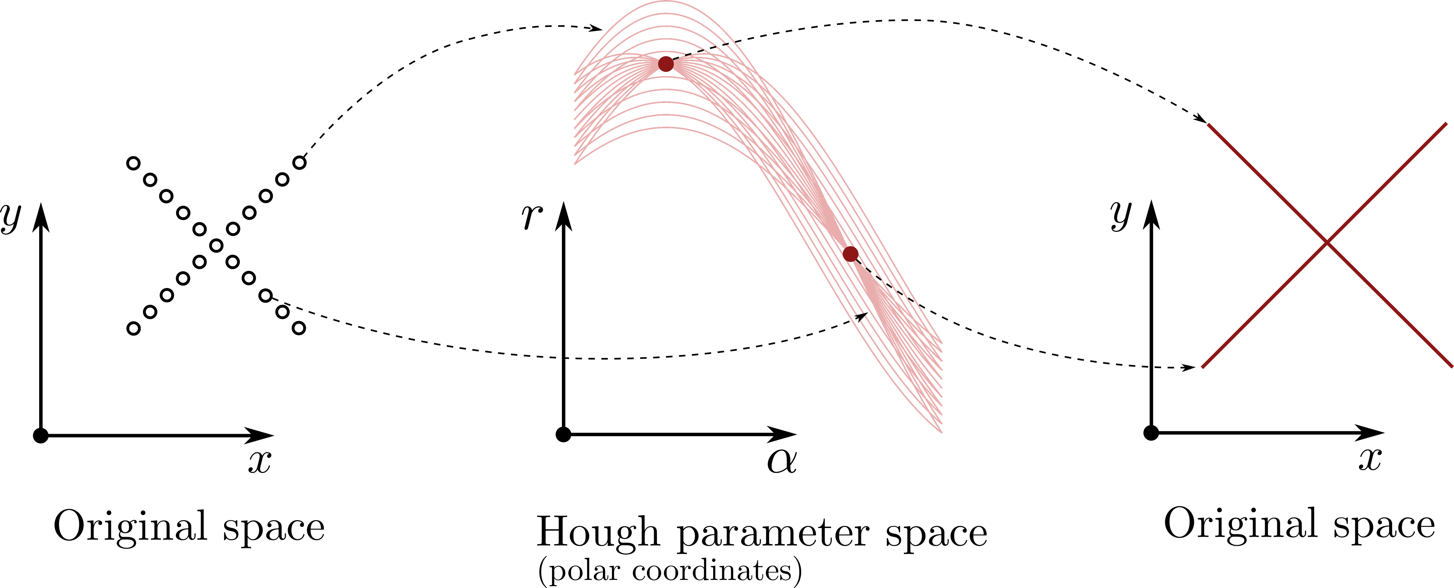
Therefore, each point, $(x,y)$ , in the original space maps to a line, $(m,b)$ , in the Hough space, as we show in Figure 8.11. The Hough transform algorithm exploits this fact by noting that two points on the same line in the original space will yield two intersecting lines in Hough space. In particular, the point where they intersect in the Hough space corresponds to the parameters $m^{*}$ and $b^{*}$ that defines the line passing between the points in the original space, as we show in Figure 8.12.

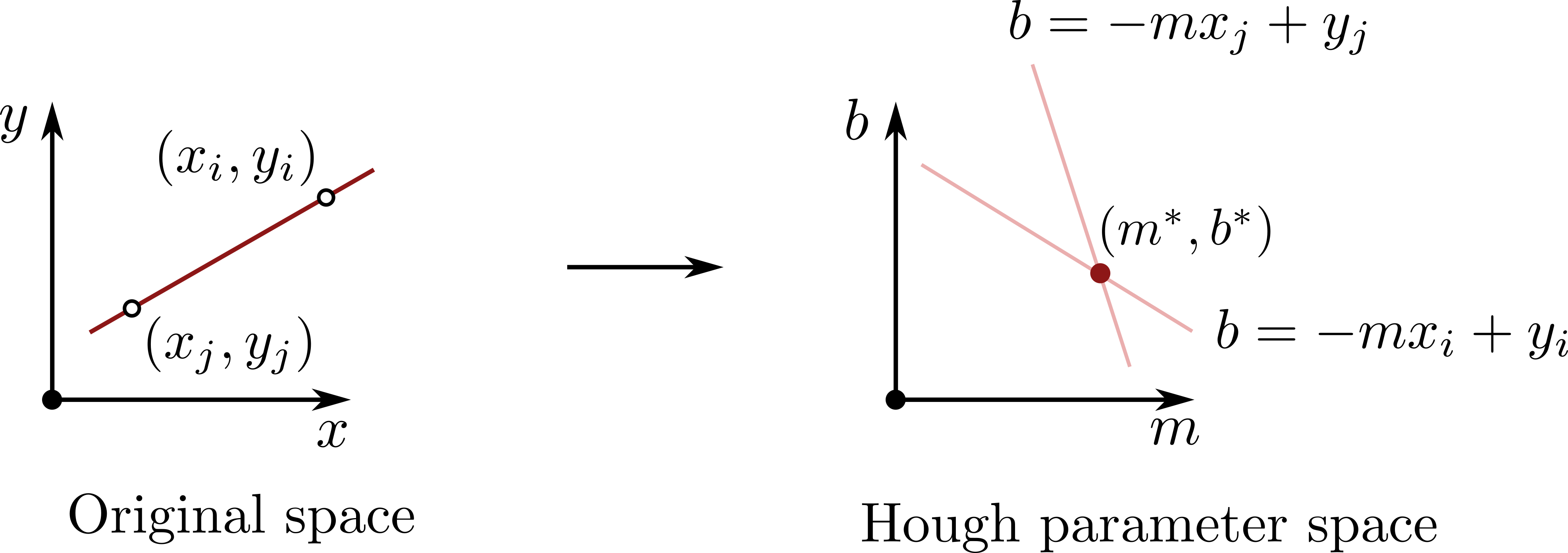
We can apply this concept to the line segmentation problem by searching in the Hough space for intersections among the lines that correspond to each point, $(x,y)$ , in the set, $S$ . In practice, we do this by discretizing the Hough space with a grid and simply counting for each grid cell the number of lines corresponding to $(x_{i},y_{i})$ points from $S$ that pass through it. We choose local maxima among the cells as lines that “fit” the data set, $S$ .

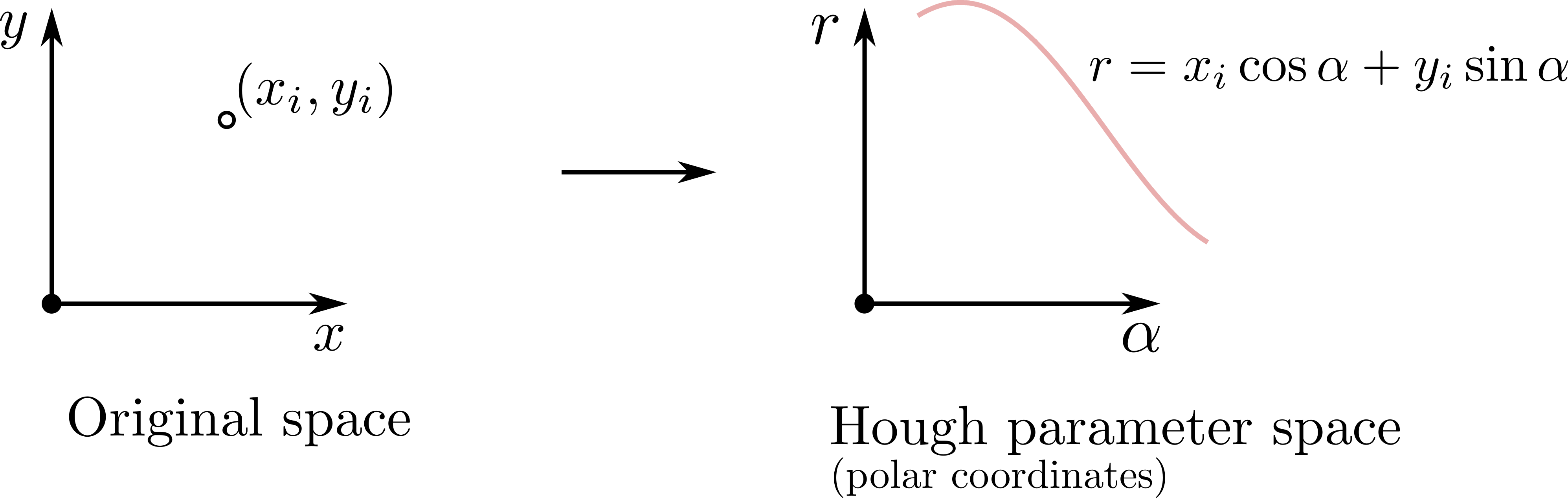
However, performing a discretization of the Hough space requires a trade-off between range and resolution, in particular because the slope, $m$ , can range from $-\infty$ to $\infty$ . Alternatively, we can use a polar coordinate representation of the Hough space which defines a line as:

x\cos\alpha+y\sin\alpha=r,

where $(\alpha,r)$ are the new line parameters. With this representation, we map a point, $(x_{i},y_{i})$ , from the original space to the polar Hough space, $(\alpha,r)$ , as a sinusoidal curve, as we show in Figure 8.13. We provide an example of the Hough transform using the polar representation in Figure 8.14.

8.2.2 Point Cloud Registration

In robotics, another important sensor modality consists of point clouds, which we can obtain from lidar or RGB-D sensors. One important consideration is to align two point clouds, generally to localize a sensor in its surroundings or to merge data from multiple viewpoints into a unified representation. We refer to this alignment problem formally as point cloud registration, which is the task of finding the geometric transformation that best aligns one point cloud to another.

The point cloud registration problem can be formulated as follows. Given a source point cloud $P\coloneqq\{p_{1},\ldots,p_{N}\}$ and a reference point cloud $Q\coloneqq\{q_{1},\ldots,q_{M}\}$ , where each $p_{i},q_{j}\in\mathbb{R}^{3}$ , our goal is to find the rigid transformation consisting of a rotation matrix $R\in SO(3)$ and translation vector $t\in\mathbb{R}^{3}$ that best aligns $P$ to $Q$ . We can express this mathematically as minimizing the error metric:

E(R,t)=\sum_{i=1}^{N}\|Rp_{i}+t-q_{i}^{*}\|^{2},

(8.7)

where $q_{i}^{*}$ denotes the closest point in $Q$ to the transformed point $Rp_{i}+t$ . This formulation leads to a challenging optimization problem because both the transformation parameters and the point correspondences are unknown.

Iterative closest point.

The Iterative Closest Point (ICP) algorithm¹⁰10. Zhang, Zhengyou. “Iterative point matching for registration of free-form curves and surfaces.” International journal of computer vision 13(2), 119–152, 1994. is a widely used method for solving the point cloud registration problem. The algorithm alternates between two steps: finding point correspondences and estimating the optimal transformation given those correspondences. We present the complete ICP algorithm in Algorithm 3 and illustrate the iterative alignment process in Figure 8.15.

Data: Source point cloud

P

, reference point cloud

Q

, initial transformation

(R_{0},t_{0})

(optional), convergence threshold

\epsilon

Result: Refined transformation

(R,t)

Initialize

(R,t)\xleftarrow{}(R_{0},t_{0})

(I,0)

if no initial guess provided

E_{\text{prev}}\xleftarrow{}\infty

repeat

// Step 1: Find correspondences

for each point $p_{i}\in P$ do

Find closest point

q_{i}^{*}\in Q

Rp_{i}+t

// Step 2: Estimate transformation

Compute optimal

(R_{\text{new}},t_{\text{new}})

that minimizes

\sum_{i=1}^{N}\|R_{\text{new}}p_{i}+t_{\text{new}}-q_{i}^{*}\|^{2}

// Step 3: Apply transformation

(R,t)\xleftarrow{}(R_{\text{new}},t_{\text{new}})

E_{\text{prev}}\xleftarrow{}E

E\xleftarrow{}\sum_{i=1}^{N}\|Rp_{i}+t-q_{i}^{*}\|^{2}

until $|E-E_{\text{prev}}|<\epsilon$ ;

Algorithm 3 Iterative Closest Point (ICP)

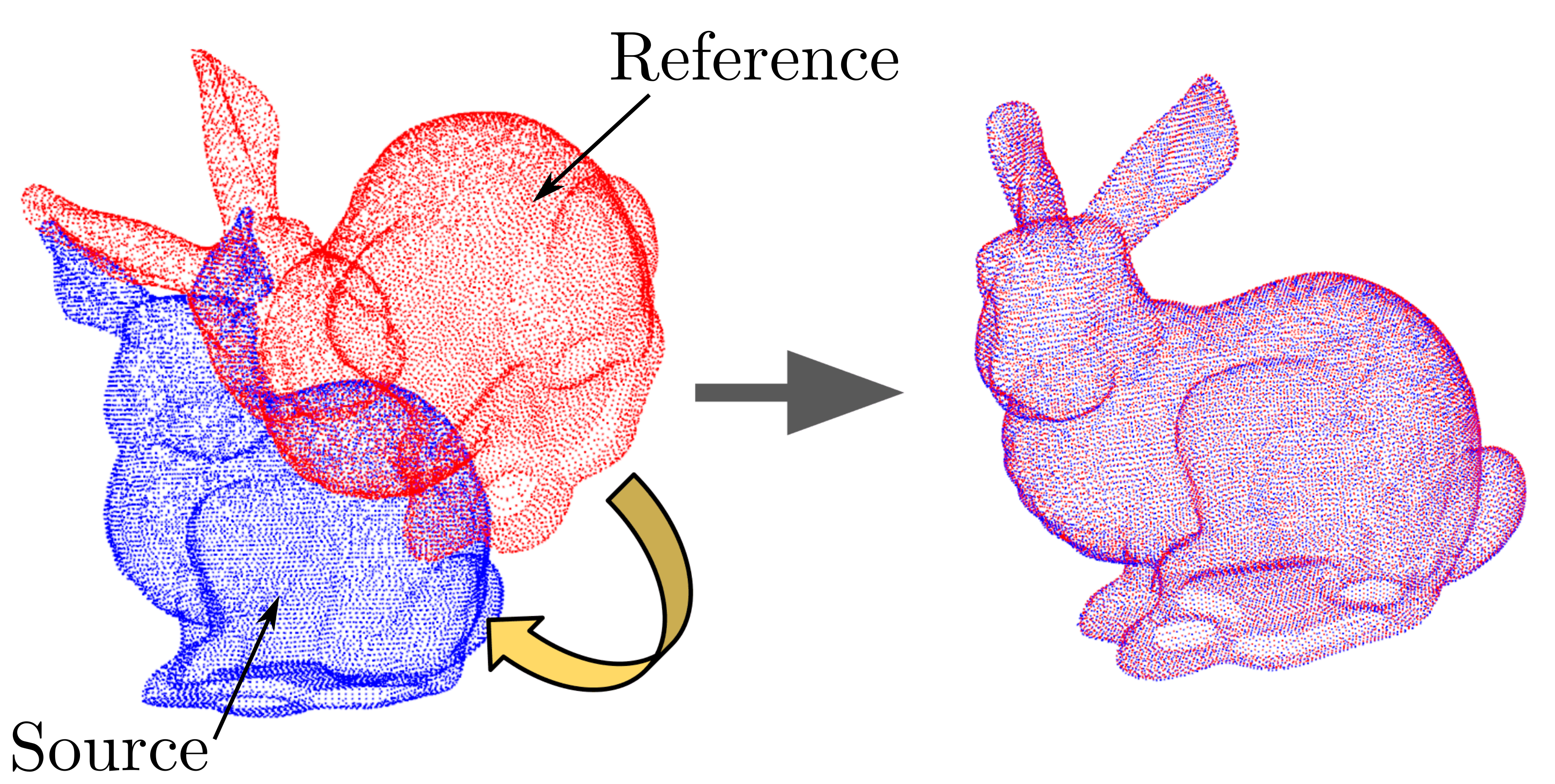
The correspondence step in ICP requires finding the nearest neighbor in $Q$ for each transformed point in $P$ . Note that while a naive implementation would require $O(NM)$ distance computations per iteration, in practice, we can accelerate this using spatial data structures such as KD-trees, which reduce the average complexity to $O(N\log M)$ . However, it is important to note that the nearest neighbor matching can produce incorrect correspondences, particularly when the point clouds are far from alignment or when they have limited overlap. The transformation estimation step computes the optimal rotation and translation given the current correspondences. This has a closed-form solution that we can obtain using singular value decomposition (SVD). First, we compute the centroids of the corresponding point sets:

\bar{p}=\frac{1}{N}\sum_{i=1}^{N}p_{i},\quad\bar{q}=\frac{1}{N}\sum_{i=1}^{N}q% _{i}^{*}.

(8.8)

Next, we construct the cross-covariance matrix:

H=\sum_{i=1}^{N}(p_{i}-\bar{p})(q_{i}^{*}-\bar{q})^{T}.

(8.9)

Computing the SVD of $H=U\Sigma V^{T}$ , the optimal rotation is $R=VU^{T}$ , and the optimal translation is $t=\bar{q}-R\bar{p}$ ^†^†margin: We must check that $\det(R)=1$ to ensure a proper rotation. If $\det(R)=-1$ , we negate the column of $V$ corresponding to the smallest singular value. .

The ICP algorithm converges when the change in error between iterations falls below a threshold $\epsilon$ , or when the change in transformation parameters is sufficiently small. The algorithm is guaranteed to monotonically decrease the alignment error and converge to a local minimum, though the quality of the final alignment is highly sensitive to the initial transformation estimate. In practice, several strategies can improve ICP’s robustness and performance, including outlier rejection methods that discard point pairs with distances exceeding a threshold to prevent corrupted correspondences from degrading the solution. As ICP remains a local optimization method, it benefits significantly from good initialization, which we can obtain from odometry, inertial sensors, or coarse global registration methods.

8.3 Feature-Based Object Detection

Another high-level information extraction task that is common in robotics is object recognition. Object recognition is the task of classifying or naming discrete objects in the world, usually based on images or video. This is a particularly challenging task because real-world scenes are commonly made up of many varying types of objects which can appear at different poses and can occlude each other. Additionally, objects within a specific class can have a large amount of variability, for example breeds of dogs or car models. In this section, we introduce common methods for feature-based object detection, namely template matching and bag of visual words.

8.3.1 Template Matching

Template matching¹¹11. Perveen, N., Kumar, D., Bhardwaj, I. “An overview on template matching methodologies and its applications.” International Journal of Research in Computer and Communication Technology 2(10), 988–995, 2013. is a machine vision technique for identifying parts of an image that match a given image pattern^†^†margin: Advanced template matching algorithms enable finding pattern occurrences regardless of their orientation and local brightness. . This approach has seen success in a variety of applications, including manufacturing quality control, mobile robotics, and more. The two primary components needed for template matching are the source image, $I$ , and a template image, $T$ .

Given a source and template image, one approach to template matching is to leverage the linear spatial correlation filters discussed earlier in this chapter. In particular, a naive approach would be to use the normalized template image as a filter mask in a correlation filter. By applying this filter mask to every pixel in the source image, the resulting output would quantify the similarity of that region of the source image to the template. This type of approach is sometimes referred to as a cross-correlation. Another approach based on linear spatial filters would be to leverage the similarity filters that compute the sum of absolute differences (SAD) metric for each pixel in the source image. Regions of the source image similar to the template would correspond to low SAD scores. The disadvantages of these approaches are that they do not handle rotations or scale changes, which are quite common in real-world applications.

One solution to the scaling issue in correlation filter based template matching is to simply re-scale the source image multiple times and perform template matching on each. We can use this concept, referred to as using image pyramids¹²12. Szeliski, R. Computer vision: algorithms and applications. Springer Science & Business Media, 2010., to accelerate object search by first using a coarser resolution image to localize the object, and then using finer resolution images for actual detection. We can build image pyramids in several ways. One naive approach is to simply eliminate some rows and columns of the image. Another approach is to first use a Gaussian smoothing filter to remove high frequency content from the image and then subsample the image. We refer to the sequence of images resulting from this approach as a Gaussian pyramid.

8.3.2 Bag of Visual Words

The key idea behind the bag of visual words^†^†margin: The model originated in natural language processing, where we consider texts such as documents, paragraphs, and sentences as collections, or “bags”, of words. approach is that we can simplify object representations by considering them as a collection of their subparts^†^†margin: For example, a bike is an object with wheels, a frame, and handlebars. , and we refer to the subparts as visual words. In this approach, we search a source image for visual words, and we create a distribution of visual words that we find in the image in the form of a histogram. We can then perform object detection by comparing this distribution to a set of training images. For example, suppose the source image contains a human face and the recognized features included eyes and a nose. Then, by comparing the distribution to training images, we would likely determine that the training images that also have eyes and a nose are also images of faces.

8.3.3 Classical Perception Approaches Today

While modern deep learning methods have revolutionized many computer vision tasks, classical perception techniques remain essential in robotics, particularly for specific instance detection and registration tasks. The fundamental methods we have discussed—feature detection, description, and matching—continue to form the backbone of many practical robotic systems. We will explore modern deep learning approaches to perception in detail in a subsequent chapter, but it is important to understand where classical methods continue to excel.

One area where classical methods remain dominant is in instance detection, where the goal is to identify and localize a specific object rather than classify object categories. For example, detecting a particular coffee cup on a cluttered desk, recognizing a specific tool in a manufacturing environment, or localizing a known landmark for robot navigation all benefit from classical approaches. Unlike category-level classification (e.g., “this is a cup”), instance detection requires identifying which specific cup among many possible cups.

The typical pipeline for instance detection leverages the classical methods we have covered:

1.

Feature Detection and Description: Extract distinctive keypoints from both the query image (the specific object to find) and the target image (the scene to search). Scale-invariant detectors like SIFT or its variants remain popular because they are robust to changes in viewpoint, scale, and illumination.
2.

Feature Matching: Match features between the query and target images using descriptor similarity. This step identifies potential correspondences between the known object and regions in the scene.
3.

Geometric Verification: Use robust estimation techniques like RANSAC to fit a geometric transformation (such as a homography or rigid body transformation) to the matched features. This step filters out incorrect matches and verifies that the pattern of features is geometrically consistent with the object model.
4.

Pose Estimation: Once verified correspondences are obtained, estimate the 3D pose of the object relative to the camera, enabling the robot to interact with or manipulate the object.

This classical pipeline offers several advantages that keep it relevant today. First, it requires only a small number of example images or even a 3D model of the specific object, whereas deep learning approaches typically require large labeled datasets. Second, it provides explicit geometric reasoning, yielding not just detection but precise pose estimation needed for robotic manipulation. Third, it is interpretable—engineers can inspect features, matches, and geometric fits to understand and debug system behavior.

Classical methods also remain important in registration problems, where the goal is to align sensor data from different viewpoints or modalities. Applications include point cloud alignment for 3D reconstruction, image stitching for panoramas, and multi-sensor fusion, which we will discuss in later chapters. The Iterative Closest Point (ICP) algorithm and feature-based registration using RANSAC continue to be workhorses in these domains. However, modern systems increasingly adopt hybrid approaches that combine classical and learning-based methods. For instance, learned feature detectors and descriptors (such as SuperPoint¹³13. DeTone, Daniel, Malisiewicz, Tomasz, Rabinovich, Andrew. “Superpoint: Self-supervised interest point detection and description.” In Proceedings of the IEEE conference on computer vision and pattern recognition workshops, 224–236, 2018.) can replace hand-crafted features like SIFT while maintaining the geometric reasoning framework. Similarly, learned feature matching networks can improve correspondence quality before geometric verification. These hybrid pipelines leverage the strengths of both paradigms: the data efficiency and geometric rigor of classical methods with the representational power of learned features.

In summary, while deep learning has transformed object classification and semantic understanding, classical perception methods remain indispensable for tasks requiring precise instance detection, geometric reasoning, and data-efficient operation. Understanding these fundamental techniques is essential for roboticists working on manipulation, localization, and any application where knowing exactly which object is where matters more than simply recognizing what category it belongs to.

8.4 Summary

In this chapter, we introduced methods for extracting various types of information from images and sensor data through a pipeline of low-level image processing and higher-level feature extraction techniques. We began with image processing fundamentals, covering filtering operations such as Gaussian smoothing for noise reduction and Sobel operators for differentiation and edge detection. We discussed the mathematical principles of correlation and convolution, along with practical implementation tricks like zero-padding. This foundation extended to feature detection, where we explored strategies for identifying semantically useful patterns like edges and corners, and the role of descriptors for representing these features.

Building on these low-level techniques, the chapter then presented methods for geometric feature extraction, focusing on the challenge of identifying structure like lines in range data. We detailed and compared three core segmentation algorithms: the fast but less robust Split-and-Merge, the robust but stochastic RANSAC, and the model-based Hough Transform. We also introduced the Iterative Closest Point (ICP) algorithm as a fundamental tool for point cloud registration. Finally, we transitioned to feature-based object detection, covering classical approaches such as template matching and the Bag of Visual Words model. We concluded by discussing the enduring relevance of these classical perception methods in modern robotics, particularly for precise instance detection and geometric verification tasks, and noted their role in hybrid systems that combine classical pipelines with learned components.

To learn more.

For a deeper exploration of the topics covered in this chapter, several key resources are available. A comprehensive introduction to the computer vision algorithms that underpin robotic perception can be found in Szeliski (2010)¹1. Szeliski, R. Computer vision: algorithms and applications. Springer Science & Business Media, 2010. and ¹⁴14. Moravec, H. P. “Towards automatic visual obstacle avoidance.” In 5th International Joint Conference on Artificial Intelligence, 1977.. The original papers on key algorithms provide invaluable insight: Fischler and Bolles (1981)²2. Fischler, Martin A., Bolles, Robert C. “Random sample consensus: a paradigm for model fitting with applications to image analysis and automated cartography.” Commun. ACM 24(6), 381–395, 1981. for RANSAC, Harris and Stephens (1988)³3. Harris, C., Stephens, M. “A combined corner and edge detector.” In 4th Alvey Vision Conference, 1988. for the corner detector, and Zhang (1994)⁴4. Zhang, Zhengyou. “Iterative point matching for registration of free-form curves and surfaces.” International journal of computer vision 13(2), 119–152, 1994. for ICP. For a deeper dive into feature descriptors, explore SIFT Lowe (2004)⁵5. Lowe, David G. “Distinctive Image Features from Scale-Invariant Keypoints.” International Journal of Computer Vision 60(2), 91–110, 2004. and its modern learned counterparts like SuperPoint ¹⁵15. DeTone, Daniel, Malisiewicz, Tomasz, Rabinovich, Andrew. “Superpoint: Self-supervised interest point detection and description.” In Proceedings of the IEEE conference on computer vision and pattern recognition workshops, 224–236, 2018.. Finally, for a broader perspective on how these classical techniques are employed in state-of-the-art systems, consult robotics and computer vision texts such as Siegwart et al. (2011)⁶6. Siegwart, R., Nourbakhsh, I. R., Scaramuzza, D. Introduction to Autonomous Mobile Robots. MIT Press, 2011..

8.5 Exercises

The starter code for the exercises provided below is available online through GitHub. To get started, download the code by running in a terminal window:

⬇

git clone https://github.com/StanfordASL/pora-exercises.git

We denote Problems requiring hand-written solutions and coding in Python with and , respectively.

Problem 1: Correlation and Gaussian Smoothing Filters

In this exercise, you will explore developing a correlation and Gaussian smoothing filter using the top-left indexing approach defined by Equation 8.3. Specifically, complete the following:

1.
First, consider an image and its zero-padded version:

$I=\begin{bmatrix}7&4&1\\ 8&5&2\\ 9&6&3\\ \end{bmatrix},\quad I_{\text{padded}}=\begin{bmatrix}0&0&0&0&0\\ 0&7&4&1&0\\ 0&8&5&2&0\\ 0&9&6&3&0\\ 0&0&0&0&0\\ \end{bmatrix}.$

Compute by hand the resulting image $I^{\prime}$ from applying the following correlation filters:
1. (a)
  
  $F=\begin{bmatrix}0&0&0\\ 0&1&0\\ 0&0&0\\ \end{bmatrix}.$
2. (b)
  
  $F=\begin{bmatrix}1&0&0\\ 0&0&0\\ 0&0&0\\ \end{bmatrix}.$
3. (c)
  
  $F=\begin{bmatrix}1&1&1\\ 0&0&0\\ -1&-1&-1\\ \end{bmatrix}.$
  
  What is this filter doing to the image? Why might this be useful in computer vision? How would this be different than the functionality of the filter:
  
  $F^{\prime}=\begin{bmatrix}-1&0&1\\ -1&0&1\\ -1&0&1\\ \end{bmatrix}.$
4. (d)
  
  $F=\frac{1}{16}\begin{bmatrix}1&2&1\\ 2&4&2\\ 1&2&1\\ \end{bmatrix}.$
  
  What is this filter doing to the image? Why might this be useful in computer vision? How would this be different than the functionality of the filter:
  
  $F^{\prime}=\frac{1}{9}\begin{bmatrix}1&1&1\\ 1&1&1\\ 1&1&1\\ \end{bmatrix}.$
2.

In the file ch08/exercises/correlation_filter.ipynb, you will now implement the correlation filter. Specifically, implement the function correlate_image using Equation 8.3. Run the provided code to see the result of your implementation for a horizontal and vertical edge detector filter applied to a test image.
3.

Also in the file ch08/exercises/correlation_filter.ipynb, implement the Gaussian smoothing filter from 8.1.1 in the function create_gaussian_filter. Run the provided code to see the result of your implementation with $\sigma=0.5$ and $\sigma=2$ . Explain the general impact of varying $\sigma$ on the resulting image.

Problem 2: Iterative Closest Point (ICP) for Point Cloud Registration

In this exercise, you will use the ICP algorithm defined in Algorithm 3 to register two different point clouds in the same reference frame. In the notebook ch08/exercises/icp.ipynb, complete the following:

1.

Run the provided code to load two point clouds: one that represents the target “full” point cloud, and another that is just a partial point cloud of the same object. The goal will be to determine the transformation that will align the partial point cloud to the target point cloud.
2.

The first step before running ICP is to get an initial transformation estimate. To accomplish this we will use the RANSAC algorithm. Explore and run the provided code to run RANSAC to get this initial estimate.
3.

Now, you will implement a basic version of the ICP algorithm. Implement the functions nearest_neighbor and icp. Run the provided code, there should now be a rough alignment between the partial and target point clouds. Note that this basic version of ICP is not necessarily robust to noise and outliers.
4.

Use the open3D library’s functions to run a more robust version of the ICP algorithm. Run the provided code to see how well the point clouds align with this implementation.

Practice · 2 notebooks

Correlation Filter Open in Colab Source
Icp Open in Colab Source