Modern computer vision has shifted from hand-crafted features to end-to-end learning with deep neural networks. Rather than manually designing feature extractors like SIFT or HOG descriptors, contemporary approaches learn hierarchical representations directly from data, achieving strong performance across diverse visual tasks. This transformation has been particularly impactful for robotics, where robust visual perception is essential for autonomous operation in complex, unstructured environments. Consider a mobile robot navigating indoors: it must process RGB images to recognize objects while interpreting 3D LiDAR point clouds to understand spatial layout and plan collision-free paths. An autonomous vehicle must fuse information from multiple cameras and LiDAR scanners, processing both 2D image grids and irregular 3D point clouds in real-time. These scenarios require neural network architectures that effectively process different data modalities. Convolutional Neural Networks (CNNs) leverage spatial locality for processing camera images. Transformers use self-attention to capture long-range dependencies and enable transfer learning. For 3D data, point-based networks like PointNet process unordered point clouds directly, while voxel-based architectures discretize 3D space into regular grids. Each architecture provides learned feature representations essential for downstream robotic tasks.
In this chapter, we explore fundamental neural network architectures for robotic perception. We begin with CNNs in Section 9.1 and Transformers in Section 9.2 for image processing, then discuss point-based approaches in Section 9.3 and voxel-based approaches in Section 9.4 for 3D sensor data. These architectural foundations serve as building blocks for the detection, segmentation, and scene understanding methods in subsequent chapters.
9.1 Convolutional Neural Networks
Convolutional neural networks (CNNs) are a type of deep learning architecture that is very common in the fields of computer vision and image processing. The architecture of a CNN contains a special structure that leverages convolution filters similar to those we discussed in Chapter 8. However, in the context of machine learning, the convolution filters embedded in the structure of a CNN are optimized for the desired task and do not require human specification, giving higher performance and reducing the amount of required manual engineering. CNN architectures comprise several main components: convolutional layers, nonlinear activations, pooling layers, and fully-connected layers. In the following sections, we discuss these components in more detail.
9.1.1 Convolution Layers
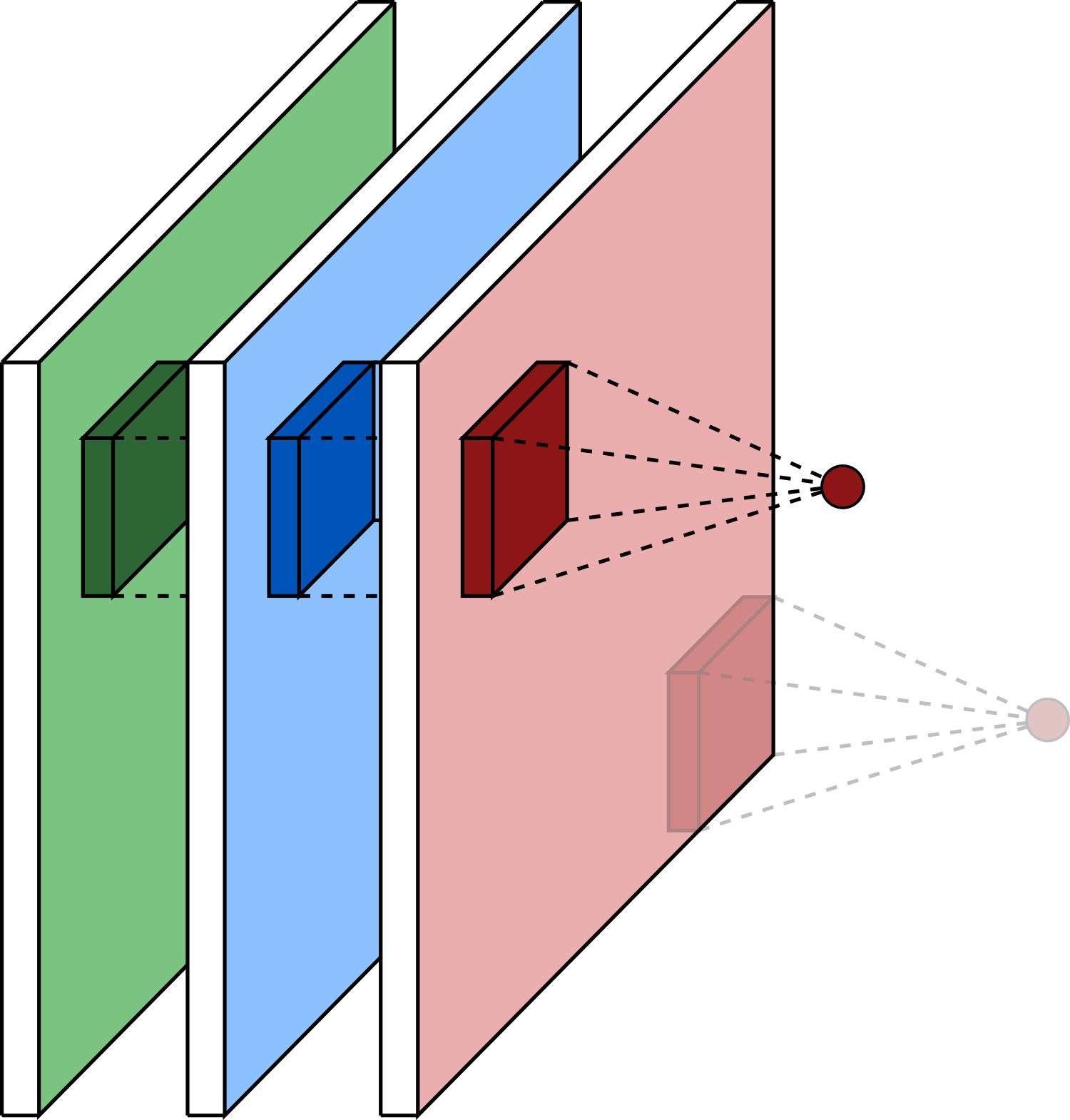
One of the main structural concepts that is unique to the architecture of a CNN is the use of convolution layers. Convolution layers exploit the underlying spatial locality structure in images by using sliding, learned filters which are often much smaller than the image itself. Mathematically, these filters perform operations in a manner similar to other linear filters used in image processing, such as Gaussian smoothing filters. For a 2D convolution operation, we can express the computation at each output location as:
| (9.1) |
where represents the spatial position in the output feature map, is the input image, is the filter with dimensions , and is the bias term. This operation slides the filter across the input, computing a weighted sum at each position. For multi-channel inputs like RGB images with channels, the convolution extends to:
where the filter now has dimension and aggregates information across all input channels to produce a single output value at each spatial location. For example, in Figure 9.1, we show how a filter is applied over an image with three color channels (red, green, and blue), so . In this case, the filter has dimension , which is vectorized to a weight vector, , with elements. The stride of the filter describes how many positions it shifts by when sliding over the input. The output of the filter is then passed through a nonlinear activation††margin: Typically a ReLU function. .
Once we have applied the filter to the entire image, the collection of outputs from the nonlinear activation function creates a new filtered image, which we typically refer to as an activation map, as shown in Figure 9.2.
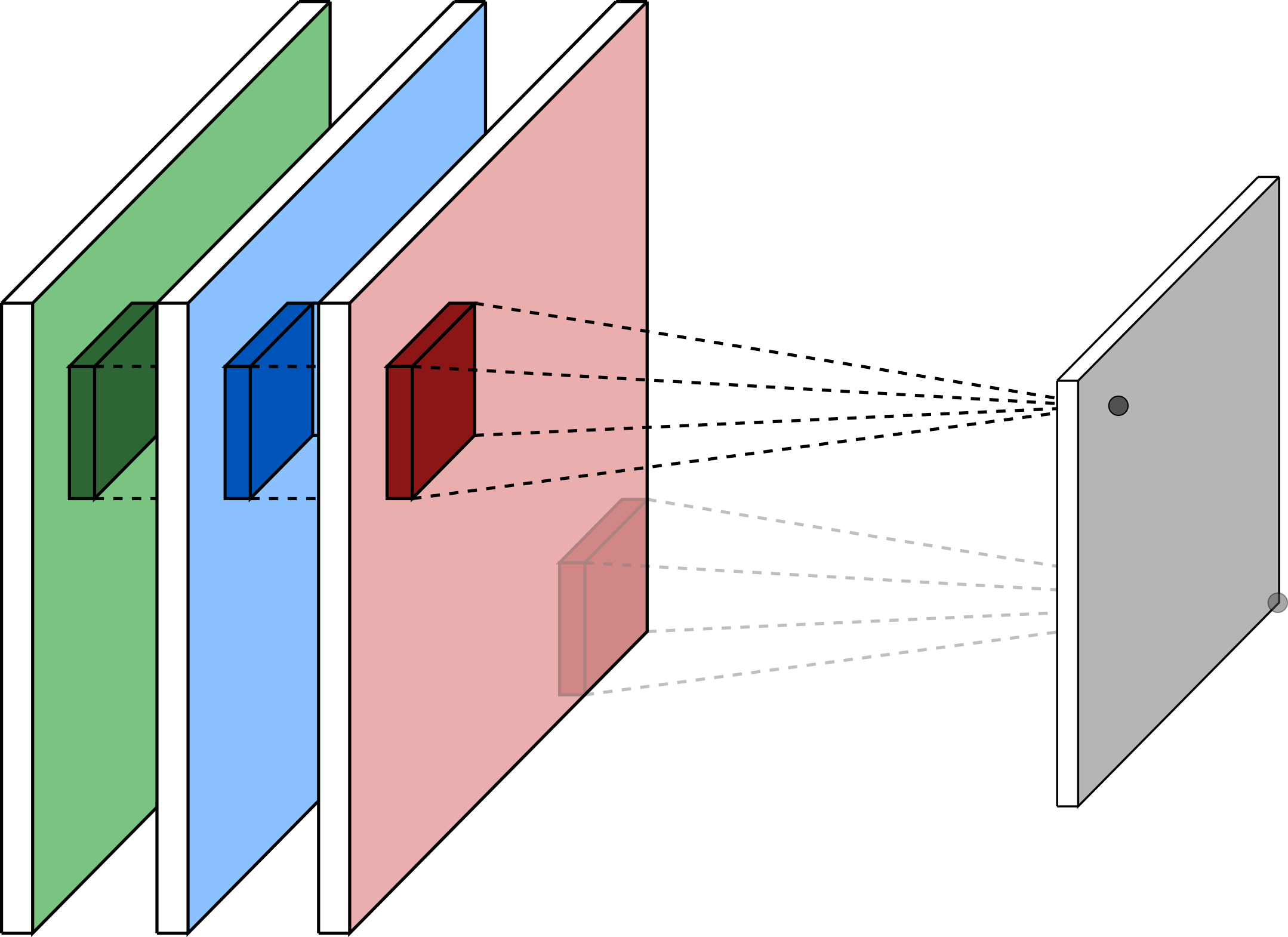
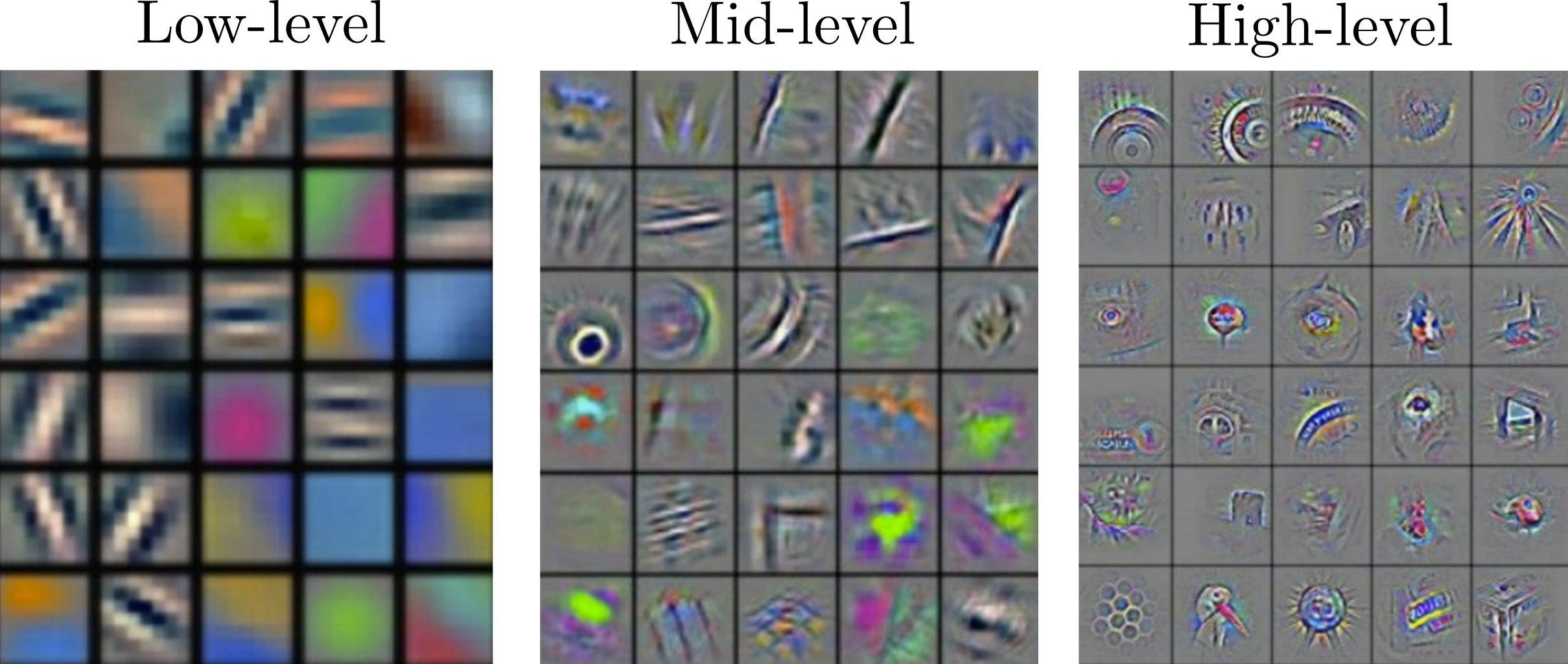
In practice, a number of different filters are usually learned in each convolution layer, which produces a corresponding number of activation maps as the output††margin: Besides the number of filters applied to the input, the width and height of the filter, the amount of padding on the input, and the stride of the filter are other hyperparameters. . This is crucial such that each filter can focus on learning one specific relevant feature. We show examples of different filters that might be learned in different convolution layers of a CNN in Figure 9.355. Zeiler, M. D., Fergus, R. “Visualizing and Understanding Convolutional Networks.” In European Conference on Computer Vision (ECCV), 818–833. Springer, 2014.. Notice that the low-level features which are learned in earlier convolution layers look a lot like edge detectors, which are more basic and fundamental features, while later convolution layers have filters that look more like actual objects.
In general, using convolution layers to exploit the spatial locality of images provides several benefits. First, parameter sharing applies the same filter parameters at all spatial locations, keeping the total number of learned parameters much smaller than fully-connected layers would require. Second, sparse interactions from having filters smaller than the image enable better detection of small, meaningful features and improve computational efficiency through fewer operations. Third, convolutional layers are equivariant to translation, meaning that convolving a shifted image produces the same result as shifting the convolution output of the original image††margin: However, convolution is not equivariant to changes in scale or rotation. , allowing feature detection regardless of position. Finally, convolutional layers can naturally handle images of varying sizes when needed.
9.1.2 Important CNN Components
In addition to convolution layers, there are several other important components that make up the architecture of a CNN.
Pooling layers.
Pooling is the second major structural component in CNNs. Pooling layers typically come after convolution layers and their nonlinear activation functions. The primary function of a pooling layer is to replace the output of the convolution layer’s activation map at particular locations with a summary statistic from other spatially local outputs. This helps make the network more robust against small translations in the input, helps improve computational efficiency by reducing the size of the input††margin: This occurs because it lowers the resolution. , and is useful in enabling the input images to vary in size††margin: The size of the pooling can be modified to keep the size of the pooling layer output constant. . The most common type of pooling is max pooling, but other types also exist, such as mean pooling. A typical max-pooling operation is shown in Figure 9.4.
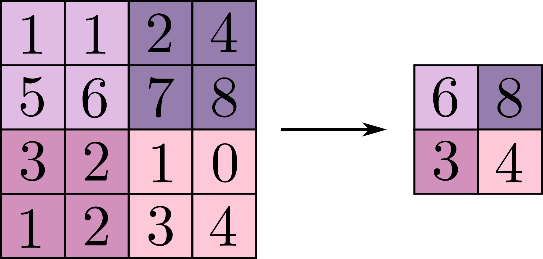
Computationally, both max and mean pooling layers operate with the same filtering idea as in the convolution layers. Specifically, a filter of width, , and height, , slides around the layer’s input with a particular stride. The difference between the two comes from the mathematical operation performed by the filter, which as their names suggest are either a maximum element or the mean over the filter. If the output of the convolution layer has activation maps, the output of the pooling layer will also have images, since the pooling filter is only applied across the spatial dimensions.
Fully connected layers.
Downstream of the convolution and pooling layers are fully connected layers. These layers make up what is essentially just a standard neural network, which is appended to the end of the network. The function of these layers is to take the output of the convolution and pooling layers, which we can think of as a highly condensed representation of the image, and perform a classification or regression. Generally, the total number of fully connected layers at the end of the CNN will only make up a fraction of the total number of layers.
CNN performance.
We can say that a CNN learns how to process images end-to-end because it essentially learns how to perform two steps simultaneously: feature extraction and classification or regression††margin: In other words, it learns the entire process from image input to the desired output. . In contrast, classical approaches to image processing use hand-engineered feature extractors. Since 2012, the performance of end-to-end learning approaches to image processing have dominated and continue to improve††margin: In some specific applications, hand-engineered features may still be better. For example, we might use engineering insight to identify a structure to the problem that a CNN could not easily learn. . This continuous improvement has generally been realized with the use of deeper networks with more parameters, and also by combining CNN architectures with other techniques such as Transformers.
9.1.3 Notable CNN Architectures
Several landmark CNN architectures have significantly advanced computer vision and demonstrated the power of deep learning.
AlexNet (2012).
AlexNet was the first deep CNN to achieve breakthrough performance on ImageNet, popularizing the use of ReLU activations and dropout regularization. It demonstrated that deeper networks could dramatically outperform traditional hand-engineered methods, marking a turning point in computer vision.
ResNet (2015).
ResNet introduced residual connections that allow information to skip layers, enabling the training of much deeper networks—up to 152 layers—without suffering from vanishing gradients. ResNet showed that network depth itself could be a key factor in improving performance, establishing residual connections as a fundamental architectural component.
YOLO (You Only Look Once).
YOLO pioneered real-time object detection by treating detection as a single regression problem rather than a multi-stage classification task. YOLO demonstrated how CNN architectures can be adapted for various computer vision tasks beyond image classification, proving that speed and accuracy need not be mutually exclusive.
These architectures have not only achieved state-of-the-art results in their respective domains but have also influenced countless subsequent designs and established important principles for CNN development.
9.2 Transformers
Transformers are deep learning architectures that have been widely applied across various domains, including natural language processing, computer vision, robotics, and more. Compared to CNNs, Transformers enforce fewer structural constraints on the input data. As long as we can organize the input into a set or sequence of tokens, it can be processed by a Transformer-based model. Since the internal structure of the Transformer is purely learned from data rather than hand-engineered, it requires less domain-specific knowledge, which makes it easier to generalize across different data modalities. Transformers are also computationally efficient and scalable due to their ability to be parallelized, allowing for extremely large models with hundreds of billions of parameters to be trained.
9.2.1 Transformer Architecture Fundamentals
The core innovation of the Transformer architecture is the self-attention mechanism, which allows the model to learn relationships between different elements in the input sequence or set. Unlike CNNs that have built-in spatial inductive biases through convolution operations, Transformers learn all spatial and semantic relationships directly from data. This flexibility comes at a cost: Transformers typically require larger datasets to achieve similar performance as architectures with stronger inductive biases, but they can also achieve superior performance when sufficient data is available.
Tokens and embeddings.
Transformers take inputs in the form of a set or sequence of tokens. A token is a numeric representation of the raw input data, expressed as a vector. The process of converting raw inputs into tokens is called tokenization, and the specific method depends on the data modality. For language tasks, a token might represent a word, subword, or character, generated through a learned dictionary lookup. For computer vision tasks, a token typically represents a patch—a square subset of the input image. For example, we can convert an image patch of size with color channels into a token vector of size by flattening the patch into a one-dimensional vector.
We then transform each token into a token embedding vector, which is a high-dimensional latent space representation. The embedding process is typically a learned linear operation that maps tokens into a space where semantically or structurally similar tokens have similar representations. We also add a positional embedding to each token embedding to encode information about the token’s position in the sequence or spatial location. This positional information is crucial because the self-attention mechanism itself is permutation-invariant and does not inherently encode order or position. For example, if a sentence places dog before cat, the model needs that ordering to capture the sentence’s correct meaning. Similarly, in vision tasks, knowing which patch came from the top-left versus bottom-right of an image provides essential spatial context††margin: Positional embeddings can be learned parameters or fixed sinusoidal functions. Learned embeddings are more flexible but require more data, while fixed embeddings can generalize to sequence lengths not seen during training. .
Once we have transformed the raw input into embedding vectors, we aggregate them as rows of an input matrix, , where is the context size††margin: In general, larger context sizes will give better performance because we can capture more unique information. However, this comes at the cost of increased computational requirements, which scale quadratically with context size due to the attention mechanism. and is the dimensionality of the embedding space.
Self-attention mechanism.
The self-attention mechanism is the key component that allows Transformers to learn relationships between all elements in the input. Each embedding vector in initially represents only a single token and does not contain contextual information from other tokens. For example, when the phrase toy car appears in a sentence, the embedding vector for car does not yet encode the modifier toy. The goal of self-attention is to allow the model to modify each embedding vector based on its relevance to all other tokens in the sequence.
Mathematically, scaled dot-product self-attention is defined as:
| (9.2) |
where is the query matrix, is the key matrix, is the value matrix, and is the output matrix. The intuition behind this formulation is that the term computes the dot product between all pairs of queries and keys, where a larger dot product indicates that a particular pair are similar or relevant to each other. We then apply the softmax function to each row of the resulting matrix to normalize the rows so that their elements sum to one††margin: The division by , where is the dimensionality of the keys and queries, helps stabilize gradients during training by preventing the dot products from becoming too large. . Finally, multiplication by the value matrix produces an output where each row is a weighted sum of all value vectors, with weights determined by the normalized attention scores.
In the Transformer architecture, we typically define these matrices as , , and , where is the input matrix with each row corresponding to one embedding vector, and , , and are matrices of learnable parameters. While we present the mathematical form using matrix notation for implementation clarity, it is often easier to reason about the transformation of a single embedding vector. Returning to our toy car example, the attention mechanism would modify the car embedding vector into a new vector that captures relevant information from other words in the sentence. The value matrix provides potential modifications corresponding to each word, and the attention scores determine which modifications to apply. In this case, the relevance weighting would likely show a strong match between car and toy, resulting in an updated embedding that represents toy car rather than a generic car.
A single attention mechanism is limited in the types of relationships it can capture, constrained by the finite parameter matrices , , and . To increase the model’s expressive capacity, Transformers use multi-head attention, which runs multiple attention mechanisms in parallel, each with unique parameter matrices , , and for , where is the number of attention heads. The outputs from all heads are concatenated and multiplied by another learned matrix to produce the final output. This allows the model to attend to different types of relationships simultaneously—for example, one head might learn syntactic relationships while another learns semantic relationships.
Transformer layer components.
Each Transformer layer consists of two main components arranged sequentially: a multi-head self-attention layer followed by a feed-forward network, with both components wrapped in residual connections and layer normalization operations, as shown in Figure 9.5.
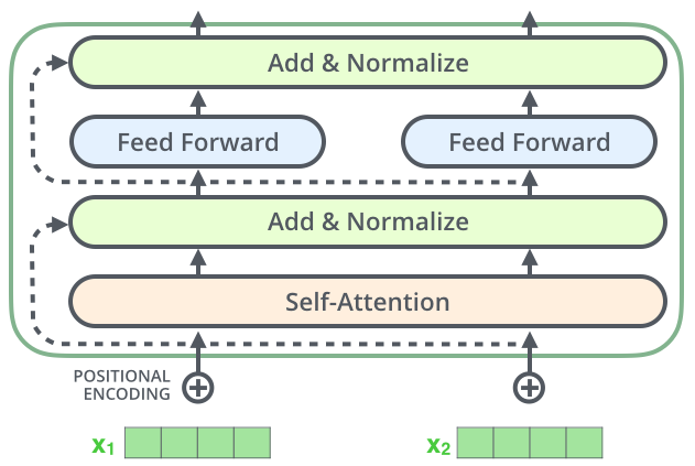
After the multi-head self-attention layer processes the input, we add the attention output back to the input in what is called a residual connection:
This residual connection allows gradients to flow more easily during training and helps the network learn identity mappings when beneficial. We then apply layer normalization to stabilize training:
Next, we pass the normalized output through a position-wise feed-forward network, typically implemented as a multi-layer perceptron (MLP). This MLP consists of two linear transformations with a non-linear activation function††margin: The ReLU or GELU activation functions are commonly used. in between:
where the MLP is applied independently to each position (each row of the input matrix). The feed-forward network typically expands the dimensionality in the first layer and then projects back to the original dimension in the second layer, allowing the network to learn complex non-linear transformations of the attention outputs. This component is followed by another residual connection and layer normalization:
A complete Transformer architecture consists of multiple such layers stacked in sequence, where the output of one layer becomes the input to the next. The depth of the network (number of stacked layers) is a key hyperparameter that significantly impacts model capacity and performance††margin: Modern Transformers can have dozens or even hundreds of layers. For example, GPT-3 has 96 layers, while some vision models use 32 or more layers. . Note that the dimensions of the inputs and outputs of each Transformer layer are typically the same (), allowing for flexible stacking of arbitrary depth.
Final linear and unembedding layer.
After passing through all Transformer layers, we must convert the final embedding representations back into a format suitable for the specific task. The unembedding layer transforms the learned embedding vectors into task-specific outputs. For classification tasks, we typically take a single embedding vector—either a special classification token or an aggregated representation of all tokens—and pass it through a linear layer followed by a softmax function:
where is the selected embedding vector, and and are learned parameters. The output is a probability distribution over the possible classes, where the vector size matches the number of classes and all elements sum to one.
For other tasks, the unembedding layer may take different forms. In sequence-to-sequence tasks like machine translation, we apply a linear transformation to each position’s embedding to predict the next token in the output sequence. In dense prediction tasks like image segmentation, we may upsample the embeddings back to the original input resolution and apply per-position classification. The specific design of the final layers depends entirely on the task requirements, while the core Transformer layers remain largely the same across different applications.
9.2.2 Vision Transformers (ViTs)
Vision Transformers66. Dosovitskiy, A., Beyer, L., Kolesnikov, A., Weissenborn, D., Zhai, X., Unterthiner, T., Dehghani, M., Minderer, M., Heigold, G., Gelly, S., Uszkoreit, J., Houlsby, N. “An Image is Worth 16x16 Words: Transformers for Image Recognition at Scale.” In International Conference on Learning Representations, 2021. represent the most important Transformer architecture for robotics practitioners, serving as the foundation for modern perception pipelines in embodied AI systems. Unlike earlier vision models that required careful hand-engineering of features and architectural components, ViTs enable end-to-end learning from raw images to task-specific outputs. They have become ubiquitous in robotic applications, from object recognition and scene understanding in autonomous navigation systems to visual representations for manipulation policies and multi-modal reasoning in household robots. The ability to pre-train ViTs on large-scale image datasets and then fine-tune them for specific robotic tasks with limited data has made them particularly valuable for real-world deployments where collecting task-specific training data is expensive or impractical.
Architecture adaptation for images.
Vision Transformers adapt the general Transformer architecture to process images by treating image patches as tokens. Given an input image of size with color channels, ViT divides the image into a grid of non-overlapping patches of size , resulting in patches. Each patch is flattened into a vector of dimension and then linearly projected to the embedding dimension through a learned embedding matrix. Common choices for patch size include or , which balance the trade-off between computational cost (smaller patches create more tokens) and the ability to capture fine-grained details††margin: For a standard image with , this creates patch tokens. .
In addition to the patch embeddings, ViT introduces a special learnable class token, denoted , which is prepended to the sequence of patch embeddings. This class token has no correspondence to any image patch but serves as a global representation that the network can use to aggregate information from all patches for classification tasks. The class token’s embedding after passing through all Transformer layers is used as the input to the final classification head. Vision Transformers use learnable 2D positional embeddings that encode each patch’s spatial location in the original image grid. Unlike 1D positional embeddings used in language models, these embeddings must capture 2D spatial structure. The standard approach uses a separate learned embedding for each position in the patch grid, which is added to the corresponding patch embedding. Alternative approaches include using sinusoidal positional encodings extended to 2D or learning relative positional biases. The complete input to the first Transformer layer is thus:
where are the linearly embedded patches and are the positional embeddings.
Training considerations.
A key characteristic of Vision Transformers is their data requirements compared to CNNs. Because ViTs lack the built-in inductive biases of convolution operations—such as translation equivariance and local connectivity—they require substantially larger training datasets to achieve comparable performance with similar model sizes. When trained on smaller datasets like ImageNet-1K (1.3 million images), ViTs typically underperform similarly-sized CNNs. However, when pre-trained on larger datasets such as ImageNet-21K (14 million images) or even larger proprietary datasets, ViTs can match or exceed CNN performance, and their performance continues to improve with dataset scale in ways that CNNs do not.
This observation has led to a standard training paradigm for ViTs: pre-training on large-scale datasets followed by fine-tuning on smaller, task-specific datasets. Pre-training can be done with supervised learning on labeled image datasets or through self-supervised methods that learn representations from unlabeled images. Self-supervised pre-training methods such as masked image modeling—where random patches are masked and the model learns to predict them—have proven particularly effective for ViTs and enable training on massive unlabeled image corpora. After pre-training, the model can be fine-tuned on downstream tasks with relatively small amounts of labeled data, often requiring only the final classification layers to be retrained while the Transformer layers remain largely fixed or are fine-tuned with small learning rates.
For robotics applications, this pre-training and fine-tuning paradigm is especially valuable. Robotic systems often operate in specialized environments with limited task-specific data, but can leverage visual representations learned from generic internet-scale image datasets. A ViT pre-trained on diverse visual data captures general-purpose features like edge detection, object recognition, and spatial relationships that transfer effectively to robotic tasks like grasping, navigation, and scene understanding.
Practical considerations.
The choice between Vision Transformers and CNNs for robotic applications involves several practical trade-offs. ViTs excel when large pre-trained models are available and when the task benefits from modeling long-range dependencies across the entire image. Their flexibility in handling variable input sizes and their ability to scale to very large model sizes make them attractive for applications where computational resources are available and high accuracy is critical. However, CNNs remain competitive or superior in scenarios with limited data, real-time constraints on resource-constrained hardware, or tasks where strong spatial inductive biases are beneficial.
Computationally, ViTs have quadratic complexity with respect to the number of patches due to the self-attention mechanism, making them more expensive than CNNs for high-resolution images. Recent variants like Swin Transformer address this by using local attention windows and hierarchical structures, combining some of the efficiency benefits of CNNs with the flexibility of Transformers. For robotics practitioners, the decision often comes down to whether pre-trained models are available for the specific visual domain, the computational budget of the deployment platform, and whether the task requires the global reasoning capabilities that attention mechanisms provide. In many modern robotic systems, hybrid approaches that combine CNN backbones for efficient feature extraction with Transformer layers for high-level reasoning have proven effective, leveraging the complementary strengths of both architectures.
9.3 Point Cloud Processing and Point-Based Networks
Robotic systems operating in 3D environments frequently rely on LiDAR sensors, depth cameras, and other sensing modalities that produce point cloud data. Point clouds represent 3D data as collections of points in space, where each point is defined by its position and may include additional attributes such as color, intensity, or surface normals††margin: Common representations include Cartesian coordinates , spherical coordinates , or cylindrical coordinates depending on the sensor type. . In autonomous driving, LiDAR sensors capture millions of points per second to create detailed 3D maps enabling real-time obstacle detection and navigation. Unlike images with regular 2D grid structure, point clouds possess unique characteristics requiring specialized neural network architectures.
9.3.1 Point Cloud Characteristics
Point clouds differ fundamentally from images in three key ways that shape neural network design. Point clouds are unordered sets with no inherent sequential or spatial ordering. A point cloud with points can be represented as where each point (typically ). Crucially, any permutation of these points represents the same geometric object, requiring neural networks to be permutation invariant.
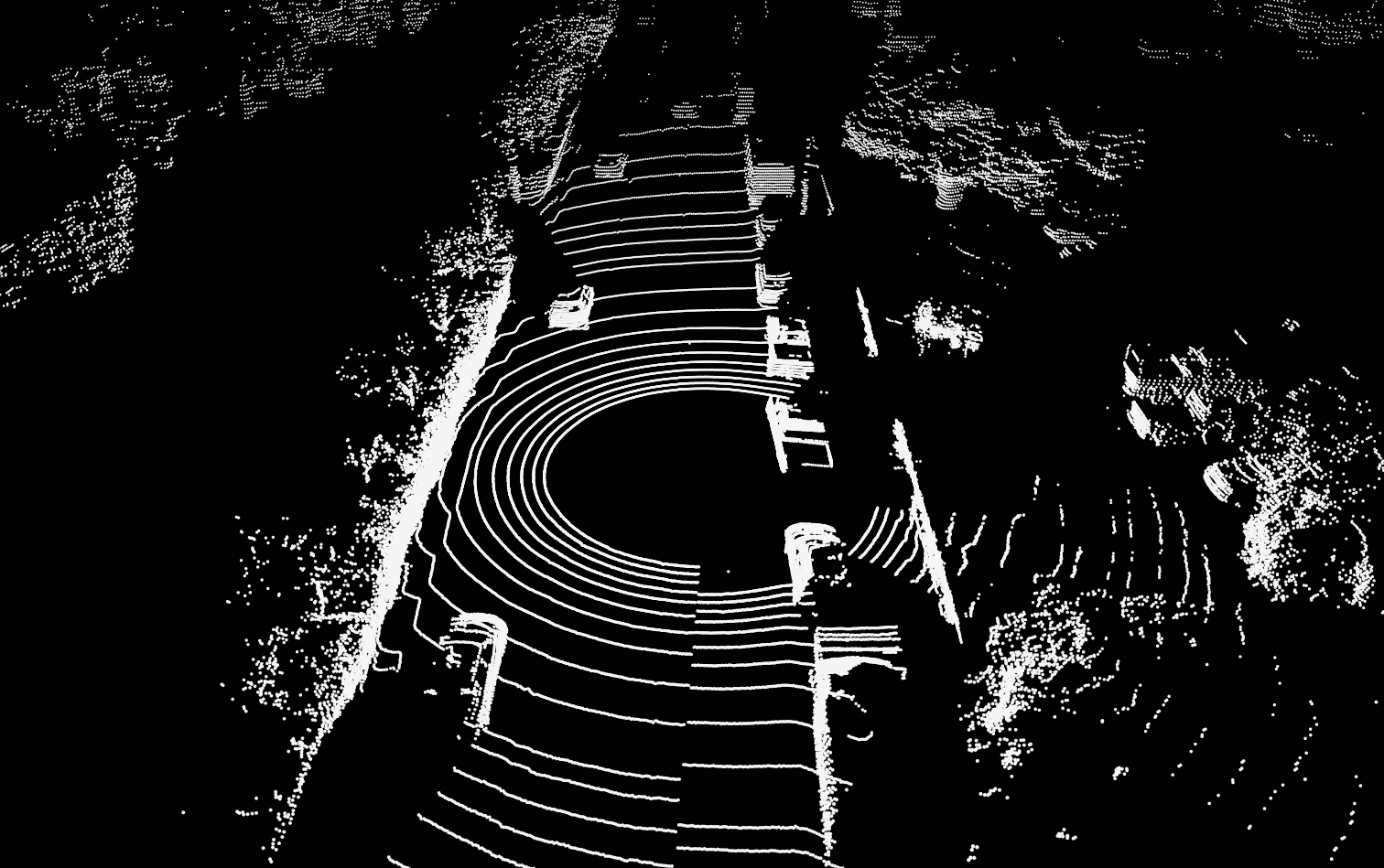
Point clouds exhibit variable cardinality, containing vastly different numbers of points across samples. While images have fixed resolution (e.g., pixels), point clouds might contain anywhere from 1,000 to 100,000 points depending on scanning resolution, sensor distance, and object complexity, posing challenges for batch processing and network design. Figure 9.6 and Figure 9.7 illustrate this variability.
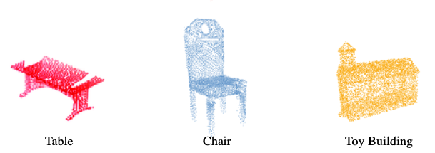
Point clouds are also sparse and irregular, with points distributed non-uniformly throughout 3D space at varying local densities determined by scanning angle, distance, and surface properties. Most 3D space contains no points, and local neighborhood structure around each point varies significantly, contrasting sharply with the dense, regular grid of image pixels.
9.3.2 PointNet Architecture
PointNet77. Qi, Charles R, Su, Hao, Mo, Kaichun, Guibas, Leonidas J. “Pointnet: Deep learning on point sets for 3d classification and segmentation.” In Proceedings of the IEEE conference on computer vision and pattern recognition, 652–660, 2017. approaches point cloud processing through several key architectural innovations that ensure permutation invariance while extracting meaningful geometric features. The architecture consists of point-wise feature extraction, symmetric aggregation functions, and spatial transformation components that work together to process unordered point sets effectively.
Point-wise multi-layer perceptrons.
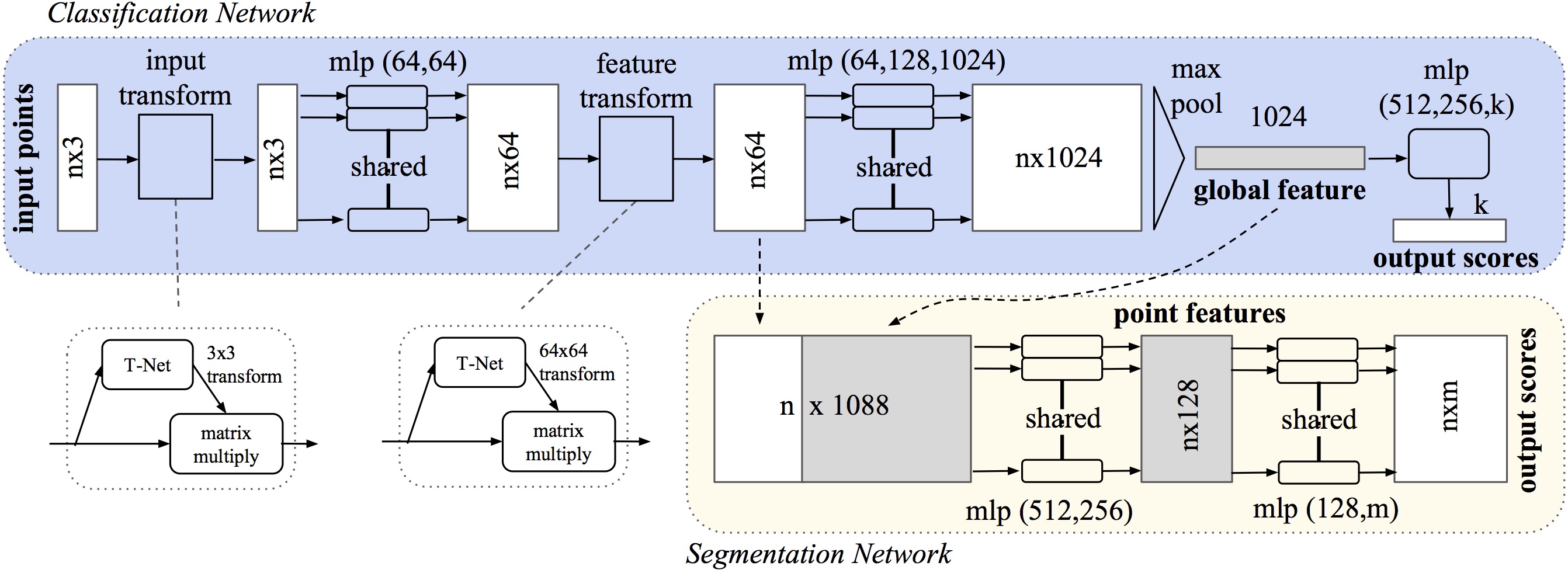
PointNet applies multi-layer perceptrons (MLPs) independently to each point in the cloud. Given points where each point represents spatial coordinates, PointNet computes:
where is the learned feature representation. This point-wise processing maintains permutation invariance because the same transformation applies to each point regardless of input order. The MLP consists of fully connected layers with ReLU activations, progressively increasing dimensionality from 3D coordinates to higher-dimensional spaces (e.g., 64, 128, 1024 dimensions). The MLP parameters are shared across all points, similar to parameter sharing in CNN filters, but without spatial locality constraints. The overall architecture is shown in Figure 9.8.
Symmetric aggregation functions.
After extracting point-wise features, PointNet must aggregate these features into a single global representation while preserving permutation invariance. This is achieved through symmetric functions that produce the same output regardless of input ordering. The most commonly used symmetric function in PointNet is the element-wise maximum:
where the max operation is applied element-wise across all feature vectors . This is provably permutation invariant because for any permutation :
While alternative symmetric functions like summation or mean could be used, max pooling has the advantage of being selective, allowing the network to focus on the most discriminative features across all points. However, this global aggregation approach means that PointNet captures only global features and may miss important local geometric structures, which motivates the hierarchical extensions in PointNet++, which we will discuss later in this section.
Transformation networks (T-Nets).
To achieve invariance to geometric transformations such as rotation and translation, PointNet incorporates transformation networks (T-Net) that learn to align point clouds to a canonical orientation. The T-Net is itself a mini-PointNet that predicts a transformation matrix :
This transformation matrix is then applied to either the input coordinates (input transform) or intermediate features (feature transform). For the input transform, aligns the spatial coordinates, while for the feature transform, normalizes the feature space. To ensure the stability of optimization, a regularization term is added to the loss function that encourages the transformation matrix to be close to orthogonal:
where denotes the Frobenius norm. This regularization prevents the transformation from becoming degenerate and helps maintain the geometric properties of the point cloud.
9.3.3 Notable Point-Based Architectures
Several landmark point-based architectures have extended PointNet’s core ideas to address its limitations and improve performance on complex 3D understanding tasks.
PointNet++.
While PointNet effectively captures global features, it struggles to learn local geometric patterns due to its reliance on global max pooling. PointNet++88. Qi, Charles Ruizhongtai, Yi, Li, Su, Hao, Guibas, Leonidas J. “Pointnet++: Deep hierarchical feature learning on point sets in a metric space.” Advances in neural information processing systems 30, 2017. addresses this limitation by introducing a hierarchical architecture that learns features at multiple scales, similar to how CNNs build hierarchical representations through multiple convolutional layers. PointNet++ introduces set abstraction layers that recursively apply PointNet to local regions. Given a point cloud with points, each set abstraction layer samples representative points (where ), groups nearby points around each representative point, and applies a PointNet to extract local features. This process creates a hierarchical pyramid of features, where early layers capture fine-grained local details and later layers capture broader geometric patterns.
Set abstraction in PointNet++ consists of three key operations: sampling, grouping, and feature extraction. Sampling uses farthest point sampling (FPS) to select representative points that provide good coverage of the entire point cloud. Given a set of points, FPS iteratively selects the point that is farthest from all previously selected points, ensuring diverse spatial coverage. Grouping then defines local regions around each selected point using either ball query (all points within radius ) or -nearest neighbors. This creates local point sets of varying sizes that capture the local geometry around each representative point. Feature extraction applies PointNet to each local region to learn features that capture local geometric patterns while maintaining permutation invariance within each region. For tasks requiring point-wise predictions like semantic segmentation, PointNet++ includes feature propagation layers that upsample features from coarser to finer resolutions. These layers use inverse distance weighted interpolation to propagate features from subsampled points back to the original point cloud:
where represents features at layer , is the distance between points, and is typically set to 2. Skip connections between corresponding abstraction and propagation layers help preserve fine-grained details, similar to U-Net architectures in image segmentation.
Dynamic graph CNN (DGCNN).
An alternative approach to processing point clouds treats them as graph structures, where points serve as nodes and edges are defined based on spatial proximity or learned relationships. Dynamic Graph Convolutional Neural Networks (DGCNN)99. Wang, Yue, Sun, Yongbin, Liu, Ziwei, Sarma, Sanjay E, Bronstein, Michael M, Solomon, Justin M. “Dynamic graph cnn for learning on point clouds.” ACM Transactions on Graphics (tog) 38(5), 1–12, 2019. exemplify this approach by constructing graphs dynamically in feature space rather than just coordinate space. DGCNN applies edge convolution operations that aggregate information from neighboring points:
where and are feature vectors of connected points, is a learnable function (typically an MLP), and the edge set is dynamically updated based on feature similarity after each layer. This dynamic graph construction allows the network to capture both geometric and semantic relationships that evolve as features are learned. The edge convolution operation differs from standard graph convolutions by explicitly modeling the edge information , which captures the relative geometric relationships between neighboring points. This approach has shown success in tasks like point cloud classification and part segmentation.
9.3.4 Applications and Limitations
After processing through these point-based architectures—PointNet’s point-wise MLPs and symmetric aggregation, PointNet++’s hierarchical set abstraction layers, or DGCNN’s dynamic graph convolutions—the networks produce rich point-wise feature representations that encode both local geometric patterns and global shape information. These learned features serve as inputs for downstream tasks including 3D object detection, semantic segmentation of points into categories like road, building, or vegetation, and instance segmentation for identifying individual objects. We will explore training methods for these detection and segmentation tasks in subsequent chapters.
Despite their effectiveness, point-based methods face computational challenges when processing large-scale point clouds. Real-world applications like autonomous driving can generate point clouds with millions of points per frame, making the complexity of neighborhood search in DGCNN or the recursive sampling in PointNet++ computationally prohibitive. Memory requirements also scale poorly, as each point must be processed individually, leading to irregular memory access patterns that are inefficient on modern GPU architectures. In the following section, we discuss voxel-based and pillar-based approaches that leverage regular grid structures for efficient 3D convolutions. By discretizing 3D space into regular voxels or vertical pillars, these methods can apply standard convolutional operations while maintaining spatial locality and enabling efficient parallel processing. This structured representation trades some geometric precision for computational efficiency and scalability, making it particularly suitable for real-time applications in autonomous driving and robotics where processing speed is critical.
9.4 Voxel-Based 3D Processing
In the previous section, we discussed that the computational limitations of point-based methods have motivated the development of grid-based approaches that discretize 3D space into regular structures, enabling the application of efficient convolutional operations. Rather than processing individual points with irregular neighborhoods, voxel-based and pillar-based methods transform point clouds into structured representations where standard CNNs can be applied. This paradigm shift trades some geometric precision for substantial computational advantages, making real-time processing of large-scale point clouds feasible for applications like autonomous driving. By leveraging the regularity of grid structures, these methods can utilize optimized convolution implementations and parallel processing capabilities of modern hardware.
9.4.1 Grid-Based Representations
Grid-based methods transform irregular point clouds into structured representations by discretizing 3D space into regular units. Two primary approaches have emerged: voxel-based representations that divide space into cubic voxels, and pillar-based††margin: Frequently used in autonomous vehicle or navigation domain, where the scene can be viewed as a 2D “map” instead of a true 3D scene, for computational efficiency. representations that use vertical columns extending through the entire height of the scene.
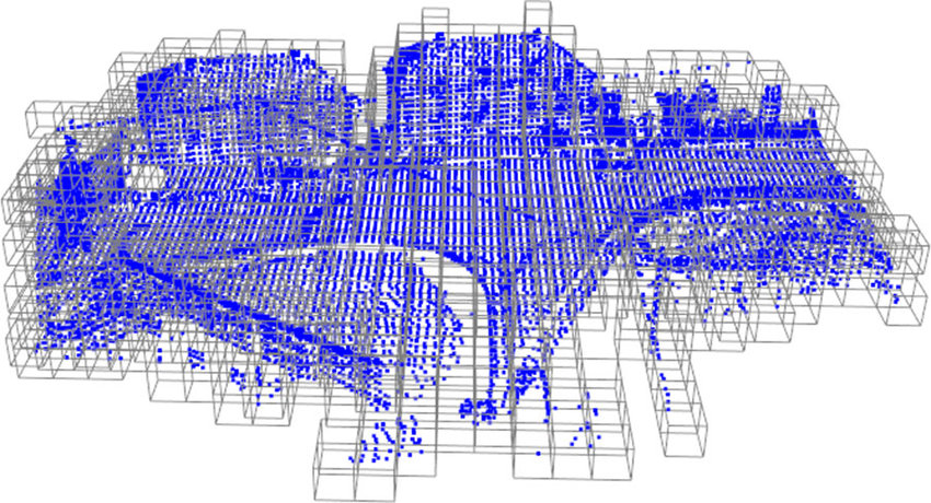
The voxel-based representation (Figure 9.9) creates a full 3D regular grid structure of size by partitioning space into cubic cells of size ††margin: In practice, these dimensions are often set to be equal, creating cubic voxels. , where each voxel can contain zero or more points from the original point cloud. This approach preserves complete spatial relationships in all three dimensions, enabling rich 3D feature learning through volumetric convolutions. Points within each voxel are aggregated into a single feature representation, typically through operations like mean pooling, max pooling, or learned aggregation functions.
In contrast, the pillar-based representation adopts a 2.5D approach, looking at the scene from a bird’s-eye view, and treats vertical columns (“pillars”) as the fundamental processing unit. The space is transformed into a 2D grid structure of size . Each pillar extends vertically through the entire height range of the point cloud, effectively collapsing the height dimension during initial processing. This approach is particularly useful in self-driving settings, where the scene processed is often very large and the reduction to 2D significantly improves computational efficiency. Points within each pillar are aggregated while preserving some height information through encoding strategies, but the primary spatial reasoning occurs in the horizontal, bird’s-eye view plane.
The choice between these representations involves significant trade-offs in computational complexity and spatial information preservation. Voxel-based methods provide richer spatial context by maintaining full 3D neighborhood relationships with memory scaling as , enabling detection of complex 3D geometric patterns but requiring computationally expensive 3D convolutions. Pillar-based approaches reduce complexity by projecting the problem into 2D with memory scaling as , enabling the use of mature 2D CNN architectures and optimized implementations, but potentially losing important vertical structure information crucial for multi-level feature detection. Both representations face spatial resolution trade-offs, where finer grids capture more geometric detail at exponentially higher computational cost, and must address sparsity challenges where most grid cells remain empty, motivating the development of sparse convolution techniques.
9.4.2 3D Convolution Fundamentals
Once point clouds are discretized into regular grid structures, we can apply convolutional operations to learn hierarchical feature representations. This section covers the fundamental operations that enable efficient processing of voxelized 3D data.
3D convolution operations.
3D Convolutional Neural Networks extend the successful principles of 2D CNNs to volumetric data by operating directly on 3D grids of voxels. While 2D convolutions slide filters across height and width dimensions of images, 3D convolutions add depth as a third spatial dimension, enabling the network to capture spatial relationships to understand the 3D scene. Specifically, a 3D convolution applies a filter of size across all three spatial dimensions of the input volume. Mathematically, for an input volume and filter , the 3D convolution operation can be expressed as:
| (9.3) |
where represents the spatial position in the output volume and is the bias term. Note that in practice, both the input and output typically have an additional channel dimension for multi-channel feature maps, and the weight is a 4D tensor that includes both spatial dimensions and input/output channel dimensions, while the bias is a vector with one element per output channel. The geometric interpretation is shown in Figure 9.10.
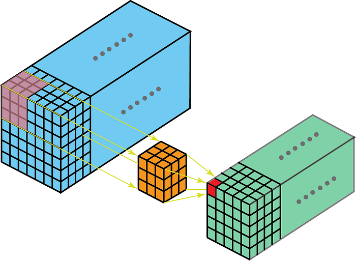
Common kernel sizes include for capturing local 3D patterns and for channel-wise feature mixing without spatial aggregation††margin: Larger kernels like can capture broader spatial context but significantly increase computational cost due to the cubic scaling of operations. . The key advantage of 3D convolutions over approaches that process 2D slices independently is their ability to learn features that span multiple depths, such as the full 3D shape of objects or volumetric textures. The receptive field in 3D grows cubically with network depth, allowing deeper layers to capture increasingly global context, though this rapid growth must be balanced against increased computational cost.
Sparse convolutions.
Real-world point clouds exhibit extreme sparsity when discretized into voxel grids. In many applications such as autonomous driving and indoor scene processing, the majority of 3D space consists of empty air or unoccupied regions. Standard dense 3D convolutions waste significant computation on empty space, making them impractical for large-scale applications. Sparse convolutions address this by computing only on occupied voxels and their neighborhoods, using efficient data structures to maintain compact representations of non-empty regions††margin: Popular implementations include spconv for PyTorch/TensorFlow and Minkowski Engine for general sparse tensor operations. .
Example 9.4.1 (Memory savings in sparse convolutions).
A typical autonomous-vehicle LiDAR scene discretized at 10cm resolution over a volume would require:
In contrast, sparse representations store only the occupied voxels, making memory usage proportional to the number of non-empty voxels rather than total grid size. The sparser the scene, the greater the memory savings.
9.4.3 Notable Voxel-Based Architectures
Several landmark architectures have demonstrated the effectiveness of grid-based representations for 3D perception tasks, particularly in autonomous driving applications where real-time performance is critical.
VoxelNet.
VoxelNet1010. Zhou, Yin, Tuzel, Oncel. “Voxelnet: End-to-end learning for point cloud based 3d object detection.” In Proceedings of the IEEE conference on computer vision and pattern recognition, 4490–4499, 2018. was one of the pioneering architectures for processing voxel-based representations. The architecture addresses the challenge of processing irregular point clouds by first voxelizing them into a 3D voxel grid, then leveraging 3D convolutions to extract features and detect objects.
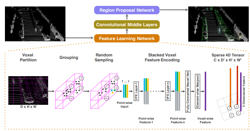
A core component of VoxelNet is its Voxel Feature Encoding (VFE) layers, which process the variable number of points within each voxel to produce fixed-size feature representations. The full architecture is shown in Figure 9.11. Given a voxel containing points , where each point includes spatial coordinates and optional reflectance intensity, the VFE layers apply point-wise multi-layer perceptrons to each point independently:
To capture contextual information within each voxel, VoxelNet augments each point with the centroid of all points in the same voxel. For a voxel containing points, the centroid is computed as , and each point is then represented as the concatenation , providing both absolute and relative spatial information. The VFE layers then aggregate features across all points in the voxel using element-wise max pooling, ensuring permutation invariance:
where is the final voxel-level feature representation. This aggregation step converts the variable-sized point sets within each voxel into fixed-size feature vectors suitable for subsequent 3D convolution operations.
After voxel feature encoding, VoxelNet applies a series of 3D convolutional middle layers to build hierarchical representations of the scene. These layers follow standard 3D CNN design principles, progressively increasing receptive field size while extracting increasingly abstract features. The sparse nature of voxel occupancy makes this stage well-suited for sparse convolution implementations to improve computational efficiency. The 3D convolutional layers aggregate information across neighboring voxels to capture larger geometric structures, build multi-scale representations through progressive downsampling, and prepare features for the final object detection stage.
PointPillars.
While VoxelNet processes full 3D voxels, PointPillars1111. Lang, Alex H, Vora, Sourabh, Caesar, Holger, Zhou, Lubing, Yang, Jiong, Beijbom, Oscar. “Pointpillars: Fast encoders for object detection from point clouds.” In Proceedings of the IEEE/CVF conference on computer vision and pattern recognition, 12697–12705, 2019. takes a different approach by using vertical pillars that extend through the entire height of the scene. The key innovation lies in the Pillar Feature Network (PFN), which encodes points within each pillar and then converts the resulting pillar features into a 2D “pseudo-image” representation. This transformation allows PointPillars to leverage mature 2D CNN architectures for subsequent processing, rather than computationally expensive 3D convolutions.
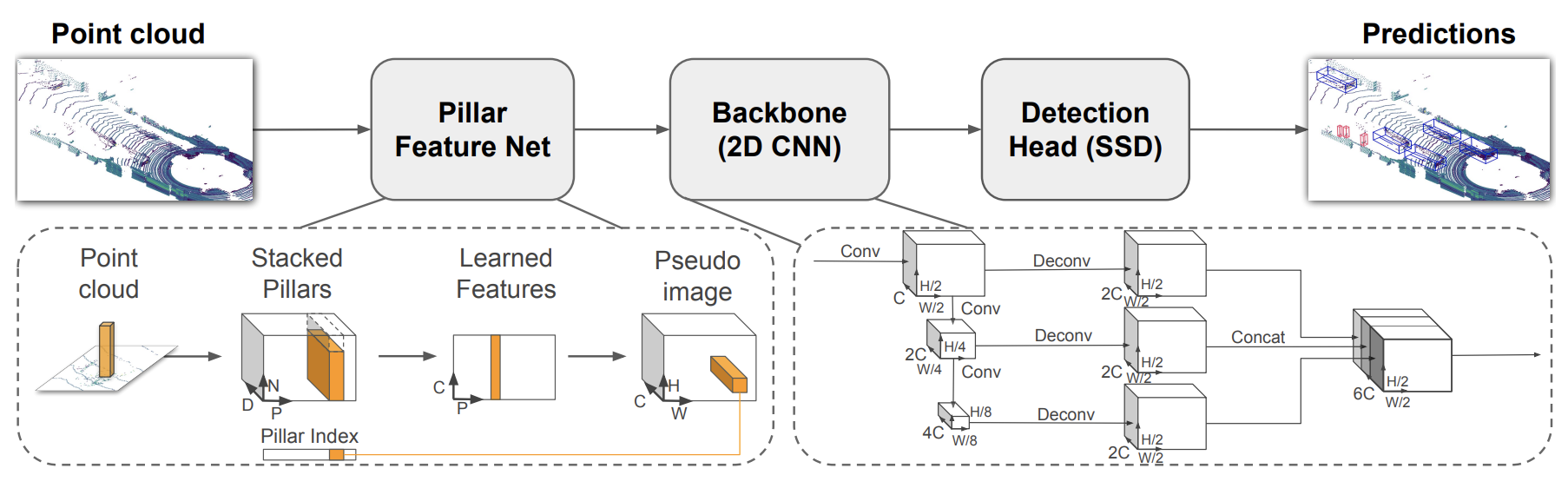
The pillar-based approach offers significant computational advantages by reducing the problem from 3D to 2.5D, enabling the use of optimized 2D convolution operations and existing hardware accelerations designed for image processing. This design choice makes PointPillars particularly suitable for real-time applications where computational efficiency is crucial, achieving inference speeds suitable for autonomous driving while maintaining competitive detection accuracy, as shown in Figure 9.12.
Other variants.
Building on the success of VoxelNet and PointPillars, several variants have been developed to further improve performance and efficiency. SECOND (Sparsely Embedded Convolutional Detection)1212. Yan, Yan, Mao, Yuxing, Li, Bo. “Second: Sparsely embedded convolutional detection.” Sensors 18(10), 3337, 2018. combines voxel-based processing with sparse convolution techniques for improved efficiency, significantly reducing computational requirements while maintaining accuracy. Voxel R-CNN extends the voxel-based approach with refined detection stages, while VoxelNet introduces architectural improvements that further push the boundaries of voxel-based 3D detection performance. Similar to point-based architectures, after processing through these voxel-based architectures—VoxelNet’s VFE layers and 3D convolutions, or PointPillars’ pillar encoding and 2D CNNs—the networks produce rich feature representations that encode geometric patterns and spatial relationships across the scene. These learned features serve as input to Region Proposal Networks (RPNs) that generate 3D bounding box proposals for object detection. The key contribution of these approaches lies in demonstrating that the entire pipeline—from raw point cloud processing to 3D object detection—can be trained end-to-end, allowing the networks to learn optimal feature representations specifically for the detection task rather than relying on hand-crafted features. We will explore the details of training object detection networks and designing appropriate loss functions in subsequent chapters on object detection and segmentation.
9.5 Summary
In this chapter, we explored fundamental neural network architectures that form the backbone of modern robotic perception, which has shifted from hand-crafted features to end-to-end learning from data. We began with Convolutional Neural Networks (CNNs), detailing their core components—convolutional layers, pooling, and fully-connected layers—that leverage spatial locality and translation equivariance for processing image data. We discussed landmark architectures like AlexNet, ResNet, and YOLO that demonstrated the power of deep, hierarchical feature learning. We then introduced the Transformer architecture, whose self-attention mechanism captures long-range dependencies without built-in spatial biases. We covered its key elements, including tokenization, positional embeddings, and multi-head attention, and focused on its adaptation to vision through Vision Transformers (ViTs), which process images as sequences of patches and excel when pre-trained on large datasets. Finally, we addressed the challenge of 3D sensor data by examining point-based networks like PointNet, which use permutation-invariant operations on point sets, and its hierarchical extension, PointNet++. We then discussed voxel-based methods, which discretize point clouds into regular grids to enable efficient 3D convolutions, as seen in VoxelNet, and pillar-based approaches like PointPillars that project data into a 2D representation for computational efficiency.
To learn more.
For a deeper exploration of the topics covered in this chapter, several key resources are available. A comprehensive foundation in deep learning concepts relevant to all architectures discussed can be found in Goodfellow et al. (2016)11. Ian Goodfellow, Yoshua Bengio, Aaron Courville. Deep Learning. MIT Press, 2016.. The seminal paper on the Transformer architecture is presented by Vaswani et al. (2017)22. Vaswani, A., Shazeer, N., Parmar, N., Uszkoreit, J., Jones, L., Gomez, A. N., Kaiser, ., Polosukhin, I. “Attention is All you Need.” In Advances in Neural Information Processing Systems. Curran Associates, Inc., 2017., while its application to vision is detailed in Dosovitskiy et al. (2021)33. Dosovitskiy, A., Beyer, L., Kolesnikov, A., Weissenborn, D., Zhai, X., Unterthiner, T., Dehghani, M., Minderer, M., Heigold, G., Gelly, S., Uszkoreit, J., Houlsby, N. “An Image is Worth 16x16 Words: Transformers for Image Recognition at Scale.” In International Conference on Learning Representations, 2021.. For in-depth studies on 3D perception, the original papers on PointNet 1313. Qi, Charles R, Su, Hao, Mo, Kaichun, Guibas, Leonidas J. “Pointnet: Deep learning on point sets for 3d classification and segmentation.” In Proceedings of the IEEE conference on computer vision and pattern recognition, 652–660, 2017. and VoxelNet 1414. Zhou, Yin, Tuzel, Oncel. “Voxelnet: End-to-end learning for point cloud based 3d object detection.” In Proceedings of the IEEE conference on computer vision and pattern recognition, 4490–4499, 2018. are essential reading. Finally, for a broader perspective on computer vision algorithms that contextualize these learning-based approaches, we refer the reader to Szeliski (2010)44. Szeliski, R. Computer vision: algorithms and applications. Springer Science & Business Media, 2010..
9.6 Exercises
The starter code for the exercises provided below is available online through GitHub. To get started, download the code by running in a terminal window:
We denote Problems requiring hand-written solutions and coding in Python with ![[Uncaptioned image]](/book-assets/deep-learning-perception/figs__write.png) and
and ![[Uncaptioned image]](/book-assets/deep-learning-perception/figs__code.png) , respectively.
, respectively.
Problem 1: Convolutional Neural Network (CNN)
In this exercise you will implement a basic convolutional neural network and use it to classify images from the CIFAR-10 dataset. The CIFAR-10 dataset consists of a large number of small RGB images of objects belonging to ten different classes. In the notebook ch09/exercises/cnn.ipynb, complete the following:
-
1.
Run the provided code to load the CIFAR-10 dataset. Take a look at some of the sample images, what is the dimension of each image?
-
2.
Complete the implementation of the SimpleCNN class to define the model architecture. Specifically, your model should have two convolution layers with ReLU activation and max pooling. Use the provided values to define the parameters of each of the features, such as the convolution kernel size and number of output channels. Following the convolution layers, your model should have two fully connected layers separated by a ReLU activation. Use the provided value to define the dimension of the hidden layer, and you should be able to determine the appropriate size of the first fully connected layer input based on the last convolution layer output size. Additionally, implement the remaining code in the training loop to train your model using the provided criterion and optimizer. Run the provided code to train your model and evaluate the model’s performance on a test dataset.
-
3.
Run the provided code to display the confusion matrix from the test dataset results. What is this showing you? Are there any surprising results or does this match your intuition?
-
4.
How many parameters does your model have in total?
Practice · 1 notebooks
- Cnn Open in Colab Source