Closed-Loop Control & Trajectory Tracking

In Chapter 2, we introduced trajectory optimization as a foundational tool for open-loop optimal control, where the objective is to compute a time-parameterized control sequence that minimizes a given cost function subject to system dynamics and constraints. Within a robot’s autonomy stack, open-loop control is often a key component, generating control sequences for tasks such as manipulation, locomotion, and navigation. However, because open-loop strategies depend only on time and not on the current system state, they are inherently vulnerable to disturbances, modeling errors, and other execution-time uncertainties.

In this chapter, we turn our attention to closed-loop optimal control. While the core elements of the problem remain the same—namely, the system dynamics, state and input constraints, and a performance criterion—the object of optimization is fundamentally different. Specifically, rather than seeking an open-loop sequence $\bm{u}(t)$ , closed-loop control aims to determine an optimal control law of the form $\bm{u}(t)=\pi(\bm{x}(t),t)$ , which explicitly depends on the current state in addition to the current time. Such closed-loop control laws are often referred to as feedback controllers or control policies.

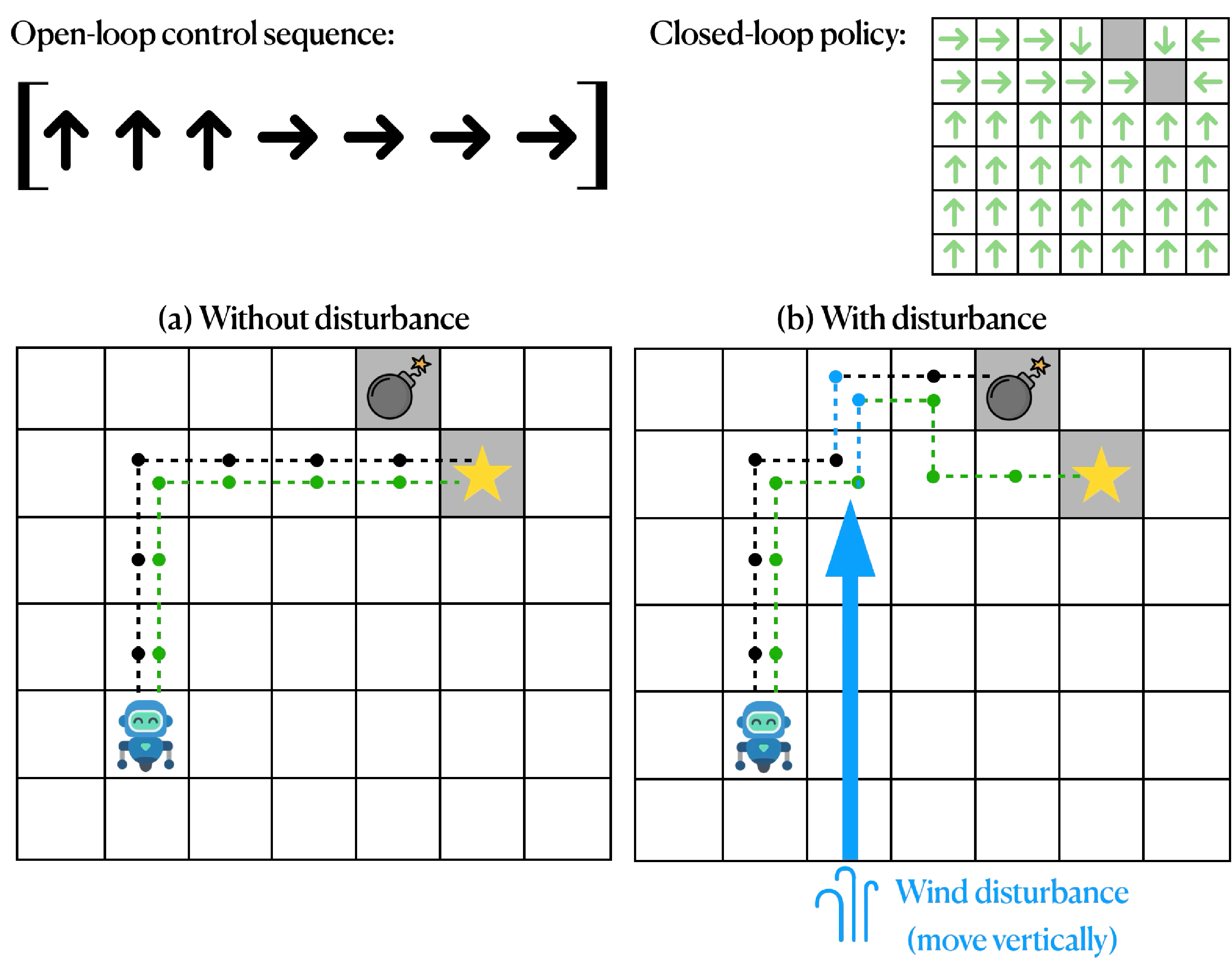
Obtaining solutions to an optimal control problem in the form of a closed-loop policy is particularly powerful, as it provides a rule prescribing optimal behavior from any state the system might encounter. Under idealized assumptions—that is, exact system models, perfect knowledge of the state, and absence of disturbances—the optimal open-loop sequence and the optimal closed-loop policy would produce identical behavior. In practice, however, such conditions are rarely met, with real systems inevitably facing model uncertainties, external disturbances, and measurement noise. In these settings, closed-loop policies offer a distinct advantage, as they continuously adapt the control input to the actual system state, thereby providing levels of robustness that are difficult to achieve through open-loop strategies (Figure 3.1).

Formally, we define a closed-loop control law as follows:

Definition 3.1 (Closed-loop control law).

A closed-loop control law is a function $\pi:\mathbb{R}^{n}\times\mathbb{R}\to\mathbb{R}^{m}$ that maps the current state^†^†margin: When the full system state is not directly measurable, closed-loop control laws can be defined based on the current measured system outputs, i.e., $\bm{u}(t)=\pi(\bm{y}(t),t)$ , where $\bm{y}(t)$ denotes the measured system output at time $t$ . In this case, the closed-loop policy is referred to as an output feedback policy. $\bm{x}(t)\in\mathbb{R}^{n}$ and time $t\in\mathbb{R}$ to a control input $\bm{u}(t)\in\mathbb{R}^{m}$ :

\bm{u}(t)=\pi(\bm{x}(t),t).

(3.1)

Despite their theoretical appeal and practical advantages, the main drawback of closed-loop control approaches is computational, as solving for an optimal closed-loop policy is generally more expensive than computing an open-loop input sequence. In practice, a useful compromise is achieved by following a two-step design, which aims to combine the strengths of both open- and closed-loop paradigms. In this scheme, one first computes a nominal reference trajectory by solving an open-loop optimal control problem, using tools such as those introduced in Chapter 2. Then, a closed-loop controller is designed to track this reference trajectory during execution. Conceptually, the resulting controller blends a feedforward term—the nominal trajectory—with a feedback term that reacts to deviations from it. As we will discuss in more depth throughout this chapter, these ideas are at the core of what is commonly referred to as trajectory tracking control.

Refer to caption — Figure 3.1: Comparison between open-loop and closed-loop control in a 2D gridworld navigation task. Without disturbances (left figure), we can see both open and closed-loop policies lead to same path, ending at the goal (star). With a wind disturbance (right figure), the fixed series of actions from the open-loop control sequence fails to take the robot to the goal after it is pushed upward by the wind. In contrast, the closed-loop policy specifies an action for each state, allowing the system to react to the disturbance and successfully reach the goal by adjusting its behavior based on the current state.

Formally, the two-step design can be expressed as:

\bm{u}(t)=\bar{\bm{u}}(t)+\pi(\bm{x}(t),\bar{\bm{x}}(t),t),

(3.2)

where $\bar{\bm{u}}(t)$ and $\bar{\bm{x}}(t)$ denote the nominal input and state trajectories, and $\pi$ is a trajectory-tracking control law ensuring that the actual trajectory remains close to the planned one despite model mismatch or disturbances.

Building on these concepts, this chapter explores key strategies for closed-loop optimal control and their application to trajectory tracking. We begin in Section 3.1 with the classical paradigm of feedback control, illustrated through the widely used proportional–integral–derivative (PID) controllers and their application to tracking, with a focus on differentially flat systems. Next, in Section 3.2, we turn to linear optimal control, focusing on the linear quadratic regulator (LQR), its key extensions, and its application to tracking control. We then discuss nonlinear optimal control problems in Section 3.3, first introducing techniques that compute optimal solutions in closed-loop form—such as the Hamilton-Jacobi-Bellman (HJB) equation and Dynamic Programming (DP)—and then showing how, for tracking purposes, linear methods can be extended to nonlinear systems through linearization. Building on this, we present how LQR ideas generalize to nonlinear optimal control through algorithms such as iterative LQR (iLQR) and differential dynamic programming (DDP), that simultaneously generate an open-loop trajectory and closed-loop tracking controller in two-step design form. Finally, in Section 3.4, we introduce model predictive control (MPC), a powerful framework that brings together ideas of open-loop and closed-loop optimal control through the framework of receding horizon optimization, and discuss how it can be applied to tracking.

3.1 Classical Feedback Control

The central goal of classical feedback control is to regulate a system’s output so that it tracks a desired reference signal. For example, in the context of an autonomous vehicle, one might want to control the vehicle’s speed to match a target velocity or maintain a specific distance from another vehicle.

The classical paradigm of feedback control is built on a simple yet powerful principle: continuously measure the system output, compare it against the desired reference, and compute corrective actions based on the resulting discrepancy, known as the error signal. These corrective inputs are then applied to the system, ensuring the output continually adjusts toward the desired behavior. For example, accelerate if the vehicle is below the target speed, or decelerate it if it is above.

Classical feedback controllers are generally designed to satisfy a set of fundamental desiderata:

•

Stability: the controller should ensure that the system remains stable. While there are several formal notions of stability, the essential requirement is that, loosely speaking, the system “is bounded in its behavior”.
•

Tracking: the controller should minimize the error between the system output and the desired reference, ensuring the system follows the commanded trajectory as closely as possible.
•

Disturbance rejection: the controller should attenuate the effects of external disturbances and measurement noise, keeping the system performance relatively unaffected by unexpected inputs.
•

Robustness: the controller should perform well despite uncertainties in the system model or parameters, ensuring reliable operation under varying conditions.

This feedback principle underlies many widely used strategies in control engineering. Among the simplest and most widely adopted strategies arising from this principle is the proportional–integral–derivative (PID) controller^†^†margin: PID control is most naturally formulated for single-input, single-output (SISO) linear systems, where the error signal is scalar. Extensions to multi-input multi-output or nonlinear systems are possible, but they often rely on heuristic tuning and provide weaker guarantees. . Despite its conceptual simplicity, PID has endured the test of time and remains a dominant tool in control engineering, from regulating temperature in industrial furnaces to stabilizing the flight of drones.

3.1.1 Structure of PID Control

A PID controller computes the control input as a weighted combination of three terms derived from the tracking error $e(t)=r(t)-y(t)$ , where $r(t)$ denotes the desired reference and $y(t)$ the measured output:

u(t)=k_{p}\,e(t)+k_{i}\int_{0}^{t}e(\tau)d\tau+k_{d}\frac{d}{dt}e(t).

(3.3)

The three terms serve complementary purposes:

•

Proportional (P): reacts immediately to deviations, producing corrective action proportional to the current error.
•

Integral (I): accumulates past error, driving steady-state error to zero.
•

Derivative (D): predicts future trends by responding to the rate of change, improving transient behavior and damping oscillations.

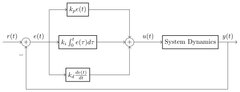
By adjusting the gains $(k_{p},k_{i},k_{d})$ , we can shape how aggressively the controller responds to disturbances, how quickly it eliminates offsets, and how smoothly it approaches the reference trajectory^†^†margin: Although tuning PID controllers is not trivial, heuristic rules such as the Ziegler–Nichols method provide systematic starting points for gain selection, but they often require further refinement in practice. . The structure of a PID controller is depicted in the block diagram in Figure 3.2. PID control is ubiquitous in industry precisely because of this simplicity: the controller can be deployed with only limited implementation effort and modest computational resources, which makes it attractive for embedded systems.

Figure 3.2: Block diagram for a PID controller in a feedback loop. The error signal $e(t)$ is computed as the difference between the reference $r(t)$ and the output $y(t)$ . The control input $u(t)$ is generated by combining the proportional, integral, and derivative terms of the error.

Example 3.1.1 (PD control of a double-integrator system).

To illustrate the mechanics of PID-type control, consider a double-integrator system with dynamics:

\dot{\bm{x}}(t)=\begin{bmatrix}0&1\\ 0&0\end{bmatrix}\bm{x}(t)+\begin{bmatrix}0\\ 1\end{bmatrix}u(t),

where $\bm{x}=\left[{x_{1},x_{2}}\right]^{\top}$ . Suppose the control objective is to regulate $x_{1}$ to the origin. A proportional–derivative controller of the form:

u(t)=-k_{p}e(t)-k_{d}\frac{de(t)}{dt},\quad e(t)=x_{1}(t),

yields closed-loop dynamics:

\dot{\bm{x}}(t)=\begin{bmatrix}0&1\\ -k_{p}&-k_{d}\end{bmatrix}\bm{x}(t),

where we have used the fact that $\dot{e}=\dot{x}_{1}=x_{2}$ . The eigenvalues of this system are:

\lambda=-\frac{k_{d}}{2}\pm\frac{1}{2}\sqrt{k_{d}^{2}-4k_{p}},

and, as a result, stability requires selecting $k_{p}$ and $k_{d}$ such that the real parts of these eigenvalues are negative; that is, $k_{p}>0$ and $k_{d}>0$ ^†^†margin: Note that a proportional controller alone, with $k_{d}=0$ , will not make the system stable since at best the eigenvalues would be purely complex, and thus the system response would be an undamped oscillation. . By appropriately tuning $k_{p}$ and $k_{d}$ , we can trade off speed of convergence against overshoot, oscillations, and sensitivity to measurement noise. For example, one might set the proportional gain $k_{p}$ to a very large value in order to drive rapid convergence to the origin. In practice, however, excessively large gains tend to amplify measurement noise and can cause the controller to behave poorly. For example, with large proportional gain $k_{p}$ , the controller may introduce oscillations, while a large derivative gain $k_{d}$ increases damping but may also slow the system’s response.

Beyond PID and PD control, classical control theory provides a rich suite of tools for analysis and design. These methods are often developed in the frequency domain^†^†margin: Frequency-domain analysis uses the Laplace transform to represent system dynamics as algebraic relations—referred to as transfer functions—rather than differential equations. , where tools such as Bode plots and the Nyquist stability criterion offer powerful ways to assess and shape system behavior. For an in-depth treatment of these topics, we refer the reader to Aström and Murray (2009)¹1. Aström, K. J., Murray, R. M. Feedback Systems. Princeton University Press, 2009..

3.1.2 Application of PID Control to Tracking Problems

Although PID controllers are most commonly associated with regulation tasks, as discussed in Example 3.1.1, the same structure introduced in Section 3.1.1 can also be employed for trajectory tracking, where the objective is to follow a time-varying nominal trajectory. In this setting, the reference signal $r(t)$ evolves over time, and the controller seeks to minimize the instantaneous tracking error $e(t)=r(t)-y(t)$ throughout the motion. While this direct application of the PID framework can perform reasonably well for simple scenarios, such as slowly varying or smooth trajectories, it remains largely heuristic, requiring ad hoc design and tuning of the gains for each specific task and system. As a result, PID-based tracking tends to be fragile and poorly generalizable, with performance degrading even under minor variations to the problem setup. There is, however, an important class of systems where PID-type control can be systematically and effectively applied to tracking: differentially flat systems.

As introduced in the referenced section, differential flatness provides a powerful framework for computing open-loop control sequences. Recall that a system with state $\bm{x}\in\mathbb{R}^{n}$ and input $\bm{u}\in\mathbb{R}^{m}$ :

\dot{\bm{x}}=f(\bm{x},\bm{u}),

is said to be differentially flat if there exists a function $\alpha$ such that:

\bm{z}=\alpha(\bm{x},\bm{u},\dot{\bm{u}},\dots,\bm{u}^{(a)}),

where $\bm{u}^{(i)}$ denotes the $i$ -th derivative of $\bm{u}$ , and such that both the system states and inputs can be expressed as algebraic functions of the flat outputs $\bm{z}\in\mathbb{R}^{m}$ and a finite number of their derivatives:

\bm{x}=\beta(\bm{z},\dot{\bm{z}},\dots,\bm{z}^{(b)}),\quad\bm{u}=\gamma(\bm{z}% ,\dot{\bm{z}},\dots,\bm{z}^{(c)}).

This structural property implies that the full system trajectory is fully determined once the flat outputs $\bm{z}(t)$ are known. In practice, we can therefore design a trajectory directly in the flat-output space—using, for example, spline interpolation or polynomial parameterizations—and reconstruct the corresponding state and control trajectories algebraically, without the need to integrate the system dynamics.

While in Chapter 2 we focused on leveraging differential flatness for open-loop trajectory generation, it is important to highlight how these systems also lend themselves naturally to trajectory tracking. In particular, differential flatness enables the trajectory tracking problem for a nonlinear system to be reduced to a linear tracking problem in the flat-output space, where classic control methods—such as PID—can be applied.

Differentially flat systems possess a particularly useful feature, as they can be feedback linearized to yield a linear system in the flat-output space. Specifically, given a differentially flat system with flat output $\bm{z}=(z_{1},\dots,z_{m})$ there exist a vector of integers $\bm{r}=(r_{1},r_{2},\dots,r_{m})$ such that:

\begin{split}\bm{x}&=\beta(z_{1},\dot{z}_{1},\dots,z_{1}^{(r_{1})},\dots,z_{m}% ,\dot{z}_{m},\dots,z_{m}^{(r_{m})}),\\ \bm{u}&=\gamma(z_{1},\dot{z}_{1},\dots,z_{1}^{(r_{1}+1)},\dots,z_{m},\dot{z}_{% m},\dots,z_{m}^{(r_{m}+1)}),\end{split}

(3.4)

and such that the system dynamics can be equivalently expressed as a linear system of the form:

\begin{split}z_{i}^{(r_{1}+1)}&=w_{1},\\ z_{2}^{(r_{2}+1)}&=w_{2},\\ \vdots\\ z_{m}^{(r_{m}+1)}&=w_{m},\end{split}

(3.5)

where $\bm{w}=(w_{1},\dots,w_{m})$ is a virtual control input that can be algebraically related to the original system inputs $\bm{u}$ ^†^†margin: For a detailed treatment of feedback linearization for differentially flat systems, we refer the reader to Levine (2009)²2. Levine, J. Analysis and Control of Nonlinear Systems: A Flatness-based Approach. Springer, 2009. and Murray (2009)³3. Murray, R. M. Optimization-Based Control. California Institute of Technology, 2009.. . The linear system in Equation 3.5 can effectively be controlled using standard linear control techniques, such as PID control.

In particular, given a reference flat output trajectory $\bm{z}_{d}=(z_{d,1},\dots,z_{d,m})$ —computed, for example, by any open-loop method—and its corresponding virtual input trajectory $\bm{w}_{d}=(w_{d,1},\dots,w_{d,m})$ , we can define the component-wise tracking error:

e_{i}\coloneqq z_{i}-z_{d,i},\quad i=1,\ldots,m,

which implies the following error dynamics:

e_{i}^{(r_{i}+1)}=w_{i}-w_{d,i}.

To ensure convergence of the tracking error to zero, we can choose the following control law:

w_{i}=w_{d,i}-\sum_{j=0}^{r_{i}}k_{i,j}e_{i}^{(j)},

which, applied to the system in Equation 3.5, yields the following closed-loop dynamics:

z_{i}^{(r_{i}+1)}=w_{d,i}-\sum_{j=0}^{r_{i}}k_{i,j}e_{i}^{(j)}.

Since $w_{d,i}=z_{d,i}^{(r_{i}+1)}$ by construction, the resulting tracking error dynamics take the form:

e_{i}^{(r_{i}+1)}+\sum_{j=0}^{r_{i}}k_{i,j}e_{i}^{(j)}=0,

where the gains $k_{i,j}>0$ are selected to enforce stability.

This procedure effectively reduces the nonlinear trajectory tracking problem to a set of decoupled linear tracking problems, one for each flat output, which can be solved using standard linear control techniques. Below, we illustrate this procedure with a concrete example.

Example 3.1.2 (PD control for a dynamically extended unicycle).

Consider the dynamically extended unicycle model introduced in the referenced item:

\begin{split}\dot{x}&=v\cos\theta,\\ \dot{y}&=v\sin\theta,\\ \dot{v}&=a,\\ \dot{\theta}&=\omega,\end{split}

with state $\bm{x}=[x,y,v,\theta]^{\top}$ and control input $\bm{u}=[a,\omega]^{\top}$ . This system is differentially flat with flat outputs $(x,y)$ and its dynamics can be expressed as:

\begin{bmatrix}\ddot{x}\\[3.0pt] \ddot{y}\end{bmatrix}=\underbrace{\begin{bmatrix}\cos\theta&-v\sin\theta\\ \sin\theta&v\cos\theta\end{bmatrix}}_{J(\theta,v)}\underbrace{\begin{bmatrix}a% \\[3.0pt] \omega\end{bmatrix}}_{\bm{u}}\coloneqq\begin{bmatrix}w_{1}\\[3.0pt] w_{2}\end{bmatrix},

(3.6)

where $\bm{w}=[w_{1},w_{2}]^{\top}$ is a virtual control input representing the flat-output accelerations, effectively transforming the system into a system of the form in Equation 3.5.

As a result, given a reference trajectory $(x_{d},y_{d})$ , we can design a feedback law for $\bm{w}$ that ensures tracking of the desired trajectory. Specifically, we can select the following PD-type virtual control:

\begin{split}w_{1}&=\ddot{x}_{d}+k_{px}(x_{d}-x)+k_{dx}(\dot{x}_{d}-\dot{x}),% \\ w_{2}&=\ddot{y}_{d}+k_{py}(y_{d}-y)+k_{dy}(\dot{y}_{d}-\dot{y}),\end{split}

(3.7)

with positive control gains $k_{px},k_{dx},k_{py},k_{dy}>0$ . Under this law, the Cartesian tracking error obeys a second-order linear differential equation:

\ddot{e}_{x}+k_{dx}\dot{e}_{x}+k_{px}e_{x}=0,\qquad\ddot{e}_{y}+k_{dy}\dot{e}_% {y}+k_{py}e_{y}=0,

ensuring that the tracking error $(e_{x},e_{y})=(x_{d}-x,y_{d}-y)$ converges exponentially to zero.

Finally, assuming the Jacobian matrix $J(\theta,v)$ is invertible, the corresponding control inputs $(a,\omega)$ can be obtained algebraically by:

\begin{bmatrix}a\\[3.0pt] \omega\end{bmatrix}=J^{-1}(\theta,v)\begin{bmatrix}w_{1}\\[3.0pt] w_{2}\end{bmatrix}.

Thus, a conceptually simple PD control law in the flat-output space translates into a nonlinear state feedback law for the original system.

3.2 Optimal Closed-loop Control for Linear Systems

Despite their widespread use and practical appeal, classical feedback controllers lack systematic methods to mathematically quantify and optimize performance. As introduced in Chapter 2, modern control theory addresses these issues by formulating controller design as an explicit optimization problem.

In this section, we focus on the linear–quadratic setting^†^†margin: That is, where the system dynamics are linear and the cost function is quadratic. , which represents one of the most elegant and widely applicable frameworks for closed-loop optimal control. Specifically, we focus on the linear quadratic regulator problem by first presenting its infinite-horizon, continuous-time formulation. Then, we discuss several important extensions of this framework—such as finite-horizon, discrete-time, and time-varying formulations—and illustrate how it can be applied to linear tracking problems.

3.2.1 The Linear Quadratic Regulator

The linear quadratic regulator (LQR) provides a principled solution to the regulation problem, where the primary objective is to drive the state of a linear system to the origin while optimally balancing state deviations against control effort^†^†margin: While this may seem like a restrictive setting at first, we will see in the remainder of this chapter that this formulation extends naturally to a wide range of practically relevant problems. . Formally, consider the linear time-invariant (LTI) system:

\dot{\bm{x}}(t)=A\bm{x}(t)+B\bm{u}(t),

(3.8)

where $A\in\mathbb{R}^{n\times n}$ and $B\in\mathbb{R}^{n\times m}$ are constant matrices. The objective is to determine a control policy $\bm{u}(t)$ that minimizes the quadratic cost functional:

J(\bm{u})=\int_{0}^{\infty}\bm{x}(t)^{\top}Q\bm{x}(t)+\bm{u}(t)^{\top}R\bm{u}(% t)dt,

(3.9)

where $Q\in\mathbb{R}^{n\times n}$ is a symmetric positive semidefinite matrix that penalizes deviations of the state from the origin and $R\in\mathbb{R}^{m\times m}$ is a symmetric positive definite matrix that penalizes control effort. Thus, in its infinite-horizon form, the LQR problem is formalized as the following optimal control problem:

\begin{split}\underset{[}{\text{minimize}}\>\quad\bm{u}]&\int_{0}^{\infty}\bm{% x}(t)^{\top}Q\bm{x}(t)+\bm{u}(t)^{\top}R\bm{u}(t)dt,\\ \text{subject to}\quad&\dot{\bm{x}}(t)=A\bm{x}(t)+B\bm{u}(t).\end{split}

(3.10)

Assuming that the pair $(A,B)$ is stabilizable and $(Q,A)$ is detectable^†^†margin: These assumptions guarantee the existence of a unique stabilizing solution to the infinite-horizon LQR problem. For formal definitions and proofs, we refer the reader to Murray (2009)⁴4. Murray, R. M. Optimization-Based Control. California Institute of Technology, 2009. and Bertsekas (2000)⁵5. Bertsekas, D. Dynamic Programming and Optimal Control. Athena Scientific, 2000.. , the LQR problem admits a unique optimal solution in the form of a stationary linear state-feedback controller:

\bm{u}(t)=-K\bm{x}(t),

(3.11)

where the optimal gain matrix $K\in\mathbb{R}^{m\times n}$ is given by:

K=R^{-1}B^{\top}P.

(3.12)

Here, $P\in\mathbb{R}^{n\times n}$ is the unique positive semidefinite solution to the continuous-time algebraic Riccati equation:

A^{\top}P+PA-PBR^{-1}B^{\top}P+Q=0.

(3.13)

The Riccati equation can be derived either through the calculus of variations—via the Pontryagin Maximum Principle introduced in Chapter 2—or through dynamic programming, using the Hamilton–Jacobi–Bellman equation^†^†margin: Both derivations lead to the Riccati equation and the same optimal linear feedback law. We refer the reader to Bertsekas (2000)⁶6. Bertsekas, D. Dynamic Programming and Optimal Control. Athena Scientific, 2000. for an in-depth treatment of both approaches. . Substituting the optimal closed-loop policy from Equation 3.11 into the system dynamics from Equation 3.8 yields the closed-loop system:

\dot{\bm{x}}(t)=(A-BK)\bm{x}(t),

(3.14)

which is guaranteed to be asymptotically stable, i.e., the eigenvalues of the matrix $A-BK$ have strictly negative real parts. Thus, the LQR problem provides a direct recipe for the regulation problem: solve the Riccati equation^†^†margin: In practice, solutions to the algebraic Riccati equation are obtained numerically using standardized software packages. Popular implementations include scipy.linalg.solve_continuous_are in Python or icare in MATLAB. , compute the optimal gain matrix $K$ , and apply the feedback law $\bm{u}(t)=-K\bm{x}(t)$ .

As a concrete example, Algorithm 3.2.1 demonstrates how to compute the optimal infinite-horizon LQR controller for a simple double integrator system with dynamics $\ddot{x}=u$ .

⬇

import numpy as np

from scipy.linalg import solve_continuous_are

# System dynamics matrices for simple double integrator

\ddot{x}

= u

A = np.array([[0, 1], [0, 0]])

B = np.array([[0], [1]])

# Define cost function matrices

Q = np.array([[1, 0], [0, 1]])

R = np.array([[1]])

# Solve the continuous algebraic Riccati equation

P = solve_continuous_are(A, B, Q, R)

# Compute optimal feedback gain matrix

K = -np.linalg.inv(R)

@

B.T

@

# Verify eigenvalues are negative (closed-loop system is stable)

eig_val, eig_vec = np.linalg.eig(A + B

@

print(eig_val)

Algorithm 3.2.1: Computing the optimal infinite-horizon LQR controller for a simple double integrator with dynamics

\ddot{x}=u

in Python. The code for this example is available in the repository github.com/StanfordASL/pora-exercises in the notebook ch03/lqr.ipynb.

Designing the cost matrices.

A central question in LQR design is how to select the cost matrices $Q$ and $R$ , as these determine the trade-off between state regulation and control effort, thereby shaping the overall closed-loop performance. For a valid solution to exist, the matrices must satisfy $Q=Q^{\top}\succeq 0$ and $R=R^{\top}\succ 0$ . To simplify the discussion, we further assume $Q=Q^{\top}\succ 0$ . Together with the stabilizability and detectability assumptions stated above, this guarantees the existence of a unique stabilizing solution to the algebraic Riccati equation. In practice, the specific choice of $Q$ and $R$ depends on the designer’s understanding of the system dynamics and performance objectives. A particularly simple and commonly adopted approach is to use diagonal weight matrices, where each diagonal element directly penalizes a corresponding state or control variable:

Q=\begin{bmatrix}q_{1}&0&\cdots&0\\ 0&q_{2}&\cdots&0\\ \vdots&\vdots&\ddots&\vdots\\ 0&0&\cdots&q_{n}\end{bmatrix},\quad R=\begin{bmatrix}r_{1}&0&\cdots&0\\ 0&r_{2}&\cdots&0\\ \vdots&\vdots&\ddots&\vdots\\ 0&0&\cdots&r_{m}\end{bmatrix},

where $q_{i}>0$ and $r_{j}>0$ for all $i=1,\ldots,n$ and $j=1,\ldots,m$ . With this choice, each diagonal entry directly specifies how strongly the corresponding (squared) state or input contributes to the overall cost. In general, states (or equivalently, control inputs) that are particularly important to regulate are assigned larger weights, ensuring that deviations in those directions are penalized more heavily. Conversely, less critical states or inputs are assigned smaller weights, reflecting their reduced influence on the system’s overall performance.

Finite-horizon formulation.

The LQR formulation can be naturally extended to the finite-horizon setting, where performance is evaluated only over a fixed time interval $[0,t_{f}]$ . In this case, the optimal control problem can be formulated as:

\begin{split}\underset{[}{\text{minimize}}\>\quad\bm{u}]&\bm{x}(t_{f})^{\top}Q% _{f}\bm{x}(t_{f})+\int_{0}^{t_{f}}\bm{x}(t)^{\top}Q\bm{x}(t)+\bm{u}(t)^{\top}R% \bm{u}(t)dt,\\ \text{subject to}\quad&\dot{\bm{x}}(t)=A\bm{x}(t)+B\bm{u}(t),\end{split}

(3.15)

where $Q_{f}\in\mathbb{R}^{n\times n}$ and $Q\in\mathbb{R}^{n\times n}$ are symmetric positive semidefinite matrices, and $R\in\mathbb{R}^{m\times m}$ is symmetric positive definite. The matrix $Q_{f}$ specifies the terminal cost, penalizing deviations of the state from the origin at the final time $t_{f}$ .

As in the infinite-horizon case, the optimal control law retains the linear form $\bm{u}(t)=-K(t)\bm{x}(t)$ , but the gain matrix becomes time-varying. Specifically, the optimal gain matrix $K(t)$ is given by:

K^{*}(t)=R^{-1}B^{\top}P(t),

(3.16)

where $P(t)$ is the positive semidefinite matrix that solves the continuous-time differential Riccati equation:

\dot{P}(t)=-A^{\top}P(t)-P(t)A+P(t)BR^{-1}B^{\top}P(t)-Q,

with terminal condition $P(t_{f})=Q_{f}$ .

As the horizon length $t_{f}$ tends to infinity, and under the standard assumptions introduced for the infinite-horizon case—namely, that $(A,B)$ is stabilizable, $(Q,A)$ is detectable, $Q=Q^{\top}\succeq 0$ , and $R=R^{\top}\succ 0$ —the solution $P(t)$ of the differential Riccati equation converges to the steady-state solution $P$ of the algebraic Riccati equation from Equation 3.13. Correspondingly, the time-varying gain matrix $K(t)$ converges to the constant gain matrix $K$ from Equation 3.12. In practice, for sufficiently long horizons, it is common to use the infinite-horizon gain directly, thereby avoiding the need to compute or store the entire gain schedule $K(t)$ .

Discrete-time LQR.

Up to this point, we have focused on continuous-time formulations. However, both the finite-horizon and infinite-horizon problems can be posed just as naturally in discrete time, where the system evolves according to the difference equation:

\bm{x}_{t+1}=A\bm{x}_{t}+B\bm{u}_{t},

(3.17)

and where, as discussed in Chapter 2, the time horizon $t_{f}$ is discretized into $N\in\mathbb{N}$ intervals $t=0,1,\ldots,N-1$ of length $\Delta t=t_{f}/N$ . In this setting, the structure of the optimal solution mirrors the continuous-time case, where the optimal state-feedback law is again linear in the state, $\bm{u}_{t}=-K_{t}\bm{x}_{t}$ , with gains obtained by solving a Riccati equation—now in its discrete form.

Specifically, the finite-horizon problem in discrete time is formulated as:

\begin{split}\underset{[}{\text{minimize}}\>\quad\bm{u}]&\bm{x}_{N}^{\top}Q_{f% }\bm{x}_{N}+\sum_{t=0}^{N-1}\bm{x}_{t}^{\top}Q\bm{x}_{t}+\bm{u}_{t}^{\top}R\bm% {u}_{t},\\ \text{subject to}\quad&\bm{x}_{t+1}=A\bm{x}_{t}+B\bm{u}_{t},\quad t=0,\ldots,N% -1,\end{split}

(3.18)

where $Q_{f}=Q_{f}^{\top}\succeq 0$ , $Q=Q^{\top}\succeq 0$ , and $R=R^{\top}\succ 0$ . The optimal solution is obtained through a backward Riccati recursion, which proceeds from the terminal condition $P_{N}=Q_{f}$ and iterates backward in time for $t=N-1,N-2,\ldots,0$ according to:

P_{t}=Q+A^{\top}P_{t+1}A-A^{\top}P_{t+1}B\bigl{(}R+B^{\top}P_{t+1}B\bigr{)}^{-% 1}B^{\top}P_{t+1}A,

(3.19)

with the corresponding feedback gain:

K_{t}=\bigl{(}R+B^{\top}P_{t+1}B\bigr{)}^{-1}B^{\top}P_{t+1}A.

(3.20)

This recursion can be viewed as the discrete-time analogue of integrating the continuous-time differential Riccati equation backward from $t_{f}$ to $0$ . At each step, $P_{t}$ is updated one stage earlier, effectively propagating future cost information back through time to determine the optimal closed-loop policy.

In the infinite-horizon setting, the problem is formulated as:

\begin{split}\underset{[}{\text{minimize}}\>\quad\bm{u}]&\sum_{t=0}^{\infty}% \bm{x}_{t}^{\top}Q\bm{x}_{t}+\bm{u}_{t}^{\top}R\bm{u}_{t},\\ \text{subject to}\quad&\bm{x}_{t+1}=A\bm{x}_{t}+B\bm{u}_{t},\end{split}

(3.21)

where $Q=Q^{\top}\succeq 0$ and $R=R^{\top}\succ 0$ . Analogous to the continuous-time case, and under the standard stabilizability and detectability conditions, the backward Riccati recursion converges—as the horizon length $t_{f}$ tends to infinity—to a steady-state matrix $P$ , which satisfies the discrete-time algebraic Riccati equation:

P=Q+A^{\top}PA-A^{\top}PB(R+B^{\top}PB)^{-1}B^{\top}PA.

(3.22)

The corresponding optimal feedback gain is then time-invariant and given by:

K=(R+B^{\top}PB)^{-1}B^{\top}PA.

(3.23)

Thus, while the overall structure of the LQR solution carries over seamlessly to discrete time, the computational machinery changes, where instead of solving a continuous-time differential or algebraic Riccati equation, one either propagates a backward recursion over a finite horizon (finite case) or solves a fixed-point equation (infinite case). This recursive viewpoint is also closely aligned with the principles of dynamic programming, which is a foundational concept in optimal control and reinforcement learning and will be discussed in more detail in the referenced item.

Below, we summarize key extensions of the LQR problem using its discrete-time formulation.

Time-varying LQR with cross-quadratic costs.

We now consider the finite-horizon, discrete-time LQR problem with both time-varying dynamics and cross-quadratic cost terms:

\begin{split}\underset{[}{\text{minimize}}\>\quad\bm{u}]&\frac{1}{2}\bm{x}_{N}% ^{\top}Q_{f}\bm{x}_{N}+\sum_{t=0}^{N-1}\left(\frac{1}{2}\bm{x}_{t}^{\top}Q_{t}% \bm{x}_{t}+\frac{1}{2}\bm{u}_{t}^{\top}R_{t}\bm{u}_{t}+\bm{x}_{t}^{\top}S_{t}% \bm{u}_{t}\right),\\ \text{subject to}\quad&\bm{x}_{t+1}=A_{t}\bm{x}_{t}+B_{t}\bm{u}_{t},\quad t=0,% \ldots,N-1,\end{split}

(3.24)

where $Q_{f}=Q_{f}^{\top}\succeq 0$ , and where $Q_{t}=Q_{t}^{\top}\succeq 0$ , $R_{t}=R_{t}^{\top}\succ 0$ , and $S_{t}$ are time-varying cost matrices. The system matrices $A_{t}$ and $B_{t}$ are also explicitly time-dependent, capturing nonstationary dynamics. This formulation extends the standard LQR problem by incorporating the cross-term matrices $S_{t}$ , which penalize state–control interactions. Such terms naturally arise when the cost of applying a control action depends on the current system state. For example, in a vehicle control scenario, the cost of applying a braking force may vary with the vehicle’s speed.

The optimal solution retains the linear feedback form $\bm{u}_{t}=-K_{t}\bm{x}_{t}$ , with:

K_{t}=(R_{t}+B_{t}^{\top}P_{t+1}B_{t})^{-1}(B_{t}^{\top}P_{t+1}A_{t}+S_{t}^{% \top}),

(3.25)

and where the matrices $P_{t}$ are obtained from the backward Riccati recursion:

P_{t}=Q_{t}+A_{t}^{\top}P_{t+1}A_{t}-(A_{t}^{\top}P_{t+1}B_{t}+S_{t})(R_{t}+B_% {t}^{\top}P_{t+1}B_{t})^{-1}(B_{t}^{\top}P_{t+1}A_{t}+S_{t}^{\top}),

(3.26)

with terminal condition $P_{t_{f}}=Q_{f}$ .

LQR with affine dynamics and quadratic and linear costs.

We now consider a more general discrete-time LQR formulation that incorporates affine dynamics together with quadratic, linear, and constant terms in the cost. Let $Q_{f}=Q_{f}^{\top}\succeq 0$ , $Q_{t}=Q_{t}^{\top}\succeq 0$ , and $R_{t}=R_{t}^{\top}\succ 0$ . The cost function is given by:

\begin{split}J(\bm{u})&=h(\bm{x}_{N})+\sum_{t=0}^{N-1}g(\bm{x}_{t},\bm{u}_{t})% ,\\ h(\bm{x}_{N})&=\frac{1}{2}\bm{x}_{N}^{\top}Q_{f}\bm{x}_{N}+\bm{q}_{f}^{\top}% \bm{x}_{N}+\alpha_{f},\\ g(\bm{x}_{t},\bm{u}_{t})&=\frac{1}{2}\bm{x}_{t}^{\top}Q_{t}\bm{x}_{t}+\frac{1}% {2}\bm{u}_{t}^{\top}R_{t}\bm{u}_{t}+\bm{x}_{t}^{\top}S_{t}\bm{u}_{t}+\\ &+\bm{q}_{t}^{\top}\bm{x}_{t}+\bm{r}_{t}^{\top}\bm{u}_{t}+\alpha_{t},\quad t=0% ,\ldots,N-1,\end{split}

(3.27)

subject to the affine dynamics:

\bm{x}_{t+1}=A_{t}\bm{x}_{t}+B_{t}\bm{u}_{t}+\bm{c}_{t}.

(3.28)

The optimal control policy can be derived using dynamic programming, yielding a time-varying affine closed-loop control law^†^†margin: In this section, we cite the result without proof and refer the reader to Bertsekas (2000)⁷7. Bertsekas, D. Dynamic Programming and Optimal Control. Athena Scientific, 2000. for a detailed derivation of the optimal solution for various LQR extensions. . To streamline notation, let us define the following intermediate quantities:

\begin{split}\eta_{t}&\coloneqq\alpha_{t}+\beta_{t+1}+p_{t+1}^{\top}\bm{c}_{t}% +\frac{1}{2}\bm{c}_{t}^{\top}P_{t+1}\bm{c}_{t},\\ h_{x,t}&\coloneqq\bm{q}_{t}+A_{t}^{\top}\left(p_{t+1}+P_{t+1}\bm{c}_{t}\right)% ,\\ h_{u,t}&\coloneqq\bm{r}_{t}+B_{t}^{\top}\left(p_{t+1}+P_{t+1}\bm{c}_{t}\right)% ,\\ H_{xx,t}&\coloneqq Q_{t}+A_{t}^{\top}P_{t+1}A_{t},\\ H_{xu,t}&\coloneqq S_{t}+A_{t}^{\top}P_{t+1}B_{t},\\ H_{uu,t}&\coloneqq R_{t}+B_{t}^{\top}P_{t+1}B_{t}.\end{split}

(3.29)

The optimal law remains affine in the state:

\bm{u}_{t}=-K_{t}\bm{x}_{t}-k_{t},

(3.30)

with parameters given recursively by:

$\displaystyle P_{N}$	$\displaystyle=Q_{f},$	(3.31)
$\displaystyle p_{N}$	$\displaystyle=\bm{q}_{f},$
$\displaystyle\beta_{N}$	$\displaystyle=\alpha_{f},$
$\displaystyle K_{t}^{*}$	$\displaystyle\coloneqq H_{uu,t}^{-1}H_{xu,t}^{\top},$
$\displaystyle k_{t}$	$\displaystyle\coloneqq H_{uu,t}^{-1}h_{u,t},$
$\displaystyle P_{t}$	$\displaystyle\coloneqq H_{xx,t}-H_{xu,t}K_{t}^{*},$
$\displaystyle p_{t}$	$\displaystyle\coloneqq h_{x,t}-H_{xu,t}k_{t},$
$\displaystyle\beta_{t}$	$\displaystyle\coloneqq\eta_{t}-\frac{1}{2}h_{u,t}^{\top}k_{t}.$

This affine–quadratic formulation generalizes the classical LQR by accommodating affine dynamics and nonhomogenous cost terms. As we will see in the remainder of this chapter, this formulation plays a central role in extending LQR techniques to nonlinear systems, where such affine and cross-linear structures naturally arise through linearization and quadratic approximation of the dynamics and cost functions.

In summary, the LQR framework represents a powerful tool for closed-loop optimal control of linear systems with quadratic costs. As we will see next, the principles underlying LQR can be extended to tackle more complex scenarios, including trajectory tracking and nonlinear dynamics.

3.2.2 Linear Tracking Problems

As discussed in the previous section, the LQR framework provides a principled solution to the regulation problem, in which the goal is to drive the system state to the origin. In many practical settings, however, tasks may extend well beyond regulation. Robotic manipulators must follow preplanned motions, autonomous vehicles must pass through waypoints, and industrial systems often operate around time-varying setpoints. In such scenarios, the control objective is one of trajectory tracking rather than regulation. Thus, restricting control design to regulation about the origin is often insufficient for many real-world applications.

The tracking problem can be naturally formulated within the two-step design paradigm introduced earlier in Equation 3.2. In the first step, an open-loop optimal control problem is solved to obtain a nominal state–control trajectory:

\left(\bar{\bm{x}}(t),\bar{\bm{u}}(t)\right),\quad t\in[0,t_{f}],

that satisfies the system dynamics and optimizes a chosen performance criterion^†^†margin: These nominal trajectories are typically computed using trajectory optimization methods, as discussed in Chapter 2. . In the second step, a closed-loop controller is designed to ensure that the actual system trajectory remains close to this nominal trajectory, compensating for disturbances, modeling errors, and measurement noise.

Formally, consider the linear system given by:

\dot{\bm{x}}(t)=A\bm{x}(t)+B\bm{u}(t),

(3.32)

and let $(\bar{\bm{x}}(t),\bar{\bm{u}}(t))$ denote a nominal trajectory we wish to track, which satisfies the same dynamics, that is:

\dot{\bar{\bm{x}}}(t)=A\bar{\bm{x}}(t)+B\bar{\bm{u}}(t).

(3.33)

We define the deviation (or error) variables as:

\delta\bm{x}(t)=\bm{x}(t)-\bar{\bm{x}}(t),\qquad\delta\bm{u}(t)=\bm{u}(t)-\bar% {\bm{u}}(t),

(3.34)

which represent the difference between the actual state and control inputs and their nominal counterparts. By using the definition of $\delta\bm{x}(t)$ in Equation 3.34 and substituting the dynamics from the referenced equation, we can derive the dynamics of the deviation variables:

	$\displaystyle\delta\dot{\bm{x}}(t)$	$\displaystyle=\dot{\bm{x}}(t)-\dot{\bar{\bm{x}}}(t)$
		$\displaystyle=[A\bm{x}(t)+B\bm{u}(t)]-[A\bar{\bm{x}}(t)+B\bar{\bm{u}}(t)]$
		$\displaystyle=A(\bm{x}(t)-\bar{\bm{x}}(t))+B(\bm{u}(t)-\bar{\bm{u}}(t))$
		$\displaystyle=A\delta\bm{x}(t)+B\delta\bm{u}(t),$

which have the same linear structure as the original system, only now expressed in terms of the deviation variables. This observation is central, as it allows the direct application of LQR techniques to the tracking problem.

LQR formulation for tracking.

Tracking performance can be naturally expressed through a quadratic cost on the deviation variables:

J(\delta\bm{u}(t))=\delta\bm{x}(t_{f})^{\top}Q_{f}\delta\bm{x}(t_{f})+\int_{0}% ^{t_{f}}\delta\bm{x}(t)^{\top}Q\delta\bm{x}(t)+\delta\bm{u}(t)^{\top}R\delta% \bm{u}(t)\,dt,

(3.35)

where $Q\succeq 0$ , $R\succ 0$ , and $Q_{f}\succeq 0$ are weighting matrices that penalize deviations of the state and control from their nominal values. The tracking problem can thus be expressed as the finite-horizon optimal control problem:

\begin{split}\underset{[}{\text{minimize}}\>\quad\delta\bm{u}]&\delta\bm{x}(t_% {f})^{\top}Q_{f}\delta\bm{x}(t_{f})+\int_{0}^{t_{f}}\delta\bm{x}(t)^{\top}Q% \delta\bm{x}(t)+\delta\bm{u}(t)^{\top}R\delta\bm{u}(t)\,dt,\\ \text{subject to}\quad&\delta\dot{\bm{x}}(t)=A\delta\bm{x}(t)+B\delta\bm{u}(t)% ,\end{split}

(3.36)

which is precisely the finite-horizon LQR problem introduced in Section 3.2.1, but now formulated in terms of the deviation variables. Therefore, all the results derived for finite-horizon LQR apply directly to this tracking formulation, and the optimal control law takes the form:

\delta\bm{u}(t)=-K(t)\delta\bm{x}(t),

(3.37)

where $K(t)$ is the time-varying optimal feedback gain obtained by solving the differential Riccati equation from Equation 3.16.

Finally, substituting the definitions of the deviation variables from Equation 3.34 yields the optimal control law in terms of the original state and control variables:

\bm{u}(t)=\bar{\bm{u}}(t)-K(t)\bigl{(}\bm{x}(t)-\bar{\bm{x}}(t)\bigr{)}.

(3.38)

This expression is a clear instantiation of the two-step design paradigm, where the control input consists of a feedforward term $\bar{\bm{u}}(t)$ , derived from the nominal trajectory, and a feedback term $-K(t)(\bm{x}(t)-\bar{\bm{x}}(t))$ that actively compensates for any deviations of the actual state from the nominal trajectory.

3.3 Optimal Closed-loop Control for Nonlinear Systems

The previous section focused on linear systems, for which the LQR framework provides elegant closed-form solutions. However, many real-world systems are inherently nonlinear, making the extension of optimal closed-loop control to nonlinear dynamics crucial for numerous practical applications.

In this section, we first briefly contextualize dynamic programming and the HJB equation—two foundational methods for deriving globally optimal closed-loop control laws in Section 3.3.1, referring the reader to the referenced item and Bertsekas (2000)⁸8. Bertsekas, D. Dynamic Programming and Optimal Control. Athena Scientific, 2000. for a more in-depth discussion. We then turn our attention to approaches that aim to leverage the structure and insights from linear optimal control to solve nonlinear optimal control problems. For trajectory-tracking, we begin by showing how the notion of linearization enables the application of LQR tracking techniques to nonlinear systems in Section 3.3.2. Finally, we extend ideas from linearization and LQR to develop algorithms that simultaneously generate an open-loop trajectory and closed-loop tracking controller in two-step design form. Specifically, we present iLQR and DDP in Section 3.3.3.

3.3.1 Dynamic Programming and the Hamilton–Jacobi–Bellman Equation

When deriving optimal closed-loop control policies for nonlinear systems, one typically distinguishes between two complementary formulations: discrete-time and continuous-time.

In the discrete-time setting, the primary tool is dynamic programming, originally developed by Richard Bellman in the 1950s. Dynamic programming provides a systematic framework for solving optimal control problems with additive cost functions and nonlinear dynamics, and it underlies numerous classical and modern optimal control algorithms, including many learning-based approaches^†^†margin: For instance, reinforcement learning algorithms discussed in the referenced item. . Intuitively, dynamic programming decomposes the optimization problem into a sequence of smaller subproblems that can be solved recursively by exploiting the principle of optimality, which informally states that for a sequence of optimal decisions, the tail of the optimal sequence is also optimal for a tail subproblem. This recursive structure leads to the celebrated Bellman equation, which dramatically simplifies the search for optimal policies by transforming the global optimization problem into a tractable sequence of smaller optimization problems.

In the continuous-time setting, the analogous formulation is given by the HJB equation. The HJB equation is a nonlinear partial differential equation whose solution enables the derivation of an optimal control law. Conceptually, it captures the infinitesimal version of the dynamic programming principle, providing a continuous-time characterization of optimality.

Both the discrete-time dynamic programming paradigm and the continuous-time HJB equation offer powerful, theoretically grounded approaches for deriving globally optimal closed-loop policies for nonlinear systems. However, they also suffer from severe computational challenges, such as the curse of dimensionality, which limit their direct applicability to high-dimensional systems.

Practical methods inspired by dynamic programming principles will be explored further in the referenced item, while for an in-depth discussion of the HJB framework, we refer the reader to Bertsekas (2000)⁹9. Bertsekas, D. Dynamic Programming and Optimal Control. Athena Scientific, 2000..

3.3.2 Linear Methods for Nonlinear Tracking Control

A common strategy for controlling nonlinear systems is to approximate their dynamics locally by a linear system and then apply linear control techniques, such as LQR tracking from Section 3.2.2. The process of approximating a nonlinear system by a linear one is called linearization and it leverages the fact that any smooth nonlinear function can be approximated locally by its first-order Taylor expansion. Below, we first describe the linearization process and then show how to apply LQR tracking to the resulting linearized system.

Linearization of nonlinear systems.

Consider the nonlinear system dynamics:

\dot{\bm{x}}(t)=f(\bm{x}(t),\bm{u}(t)),

(3.39)

where $f:\mathbb{R}^{n}\times\mathbb{R}^{m}\to\mathbb{R}^{n}$ is a smooth nonlinear function that governs the system’s evolution. Let $\left(\bar{\bm{x}}(t),\bar{\bm{u}}(t)\right)$ denote a nominal state and control trajectory that satisfies the dynamics, that is:

\dot{\bar{\bm{x}}}(t)=f(\bar{\bm{x}}(t),\bar{\bm{u}}(t)).

(3.40)

For the purposes of trajectory-tracking, we are interested in controlling the system so that it remains close to this nominal trajectory, i.e., such that the state deviations $\delta\bm{x}(t)=\bm{x}(t)-\bar{\bm{x}}(t)$ are small. As in the linear case (see Section 3.2.2), let us first derive the dynamics of these deviation variables and then design a controller to stabilize them around zero.

Using the referenced equation, the deviation dynamics can be written as:

\delta\dot{\bm{x}}(t)=\dot{\bm{x}}(t)-\dot{\bar{\bm{x}}}(t)=f(\bm{x}(t),\bm{u}% (t))-f(\bar{\bm{x}}(t),\bar{\bm{u}}(t)),

(3.41)

where, to approximate the right-hand side, we can linearize the nonlinear function $f$ around the nominal trajectory. Specifically, assuming that the deviations $\delta\bm{x}(t)$ and $\delta\bm{u}(t)=\bm{u}(t)-\bar{\bm{u}}(t)$ are small, a first-order Taylor expansion of $f$ yields:

f(\bm{x}(t),\bm{u}(t))\approx f(\bar{\bm{x}}(t),\bar{\bm{u}}(t))+\underbrace{% \frac{\partial f}{\partial\bm{x}}(\bar{\bm{x}}(t),\bar{\bm{u}}(t))}_{\coloneqq A% (t)}\delta\bm{x}(t)+\underbrace{\frac{\partial f}{\partial\bm{u}}(\bar{\bm{x}}% (t),\bar{\bm{u}}(t))}_{\coloneqq B(t)}\delta\bm{u}(t),

(3.42)

where $A(t)\in\mathbb{R}^{n\times n}$ and $B(t)\in\mathbb{R}^{n\times m}$ are the Jacobians of $f$ with respect to the state and control input, evaluated along the nominal trajectory, that is, at $(\bar{\bm{x}}(t),\bar{\bm{u}}(t))$ .

Substituting the approximation from Equation 3.42 into Equation 3.41, we obtain:

\begin{split}\delta\dot{\bm{x}}(t)&\approx\bigl{[}f(\bar{\bm{x}}(t),\bar{\bm{u% }}(t))+A(t)\,\delta\bm{x}(t)+B(t)\,\delta\bm{u}(t)\bigr{]}-f(\bar{\bm{x}}(t),% \bar{\bm{u}}(t)),\end{split}

(3.43)

which yields the linearized dynamics for the deviation variables:

\delta\dot{\bm{x}}(t)\approx A(t)\delta\bm{x}(t)+B(t)\delta\bm{u}(t).

(3.44)

Applying LQR tracking to the linearized system.

Once in this form, standard linear control techniques, such as the LQR tracking framework, can be directly applied to design a feedback controller that stabilizes the deviation dynamics around zero. For instance, applying the finite-horizon LQR tracking framework from Section 3.2.2 yields the optimal feedback law:

\delta\bm{u}(t)=-K(t)\,\delta\bm{x}(t).

which, expressed in the original variables, gives the closed-loop controller:

\bm{u}(t)=\bar{\bm{u}}(t)-K(t)\bigl{(}\bm{x}(t)-\bar{\bm{x}}(t)\bigr{)},

where $K(t)$ is the time-varying feedback gain computed by solving the differential Riccati equation associated with the linearized system.

Linearizing around an equilibrium point.

A particularly important special case arises when the nominal trajectory corresponds to a constant equilibrium $(\bar{\bm{x}},\bar{\bm{u}})$ . A state $\bar{\bm{x}}$ is referred to as an equilibrium if there exists a control input $\bar{\bm{u}}$ (called the equilibrium input) such that $f(\bar{\bm{x}},\bar{\bm{u}})=0$ . In other words, if the system is initialized at $\bar{\bm{x}}$ and the constant input $\bar{\bm{u}}$ is applied for all $t\geq t_{0}$ , the state will remain fixed at $\bar{\bm{x}}$ indefinitely. Linearizing about $(\bar{\bm{x}},\bar{\bm{u}})$ produces a system of the form in Equation 3.44, where $A$ and $B$ would be constant matrices (not time-varying) evaluated at the equilibrium.

Local validity of linearization.

It is important to highlight that linearization provides only a local approximation, and the linearized model accurately captures the system dynamics only in a neighborhood of the nominal trajectory. If the state deviates significantly from $\bar{\bm{x}}(t)$ , the linear approximation may no longer hold, and the resulting controller may perform poorly or even destabilize the system.

Below, we illustrate the linearization process with a concrete example.

Example 3.3.1 (Inverted pendulum).

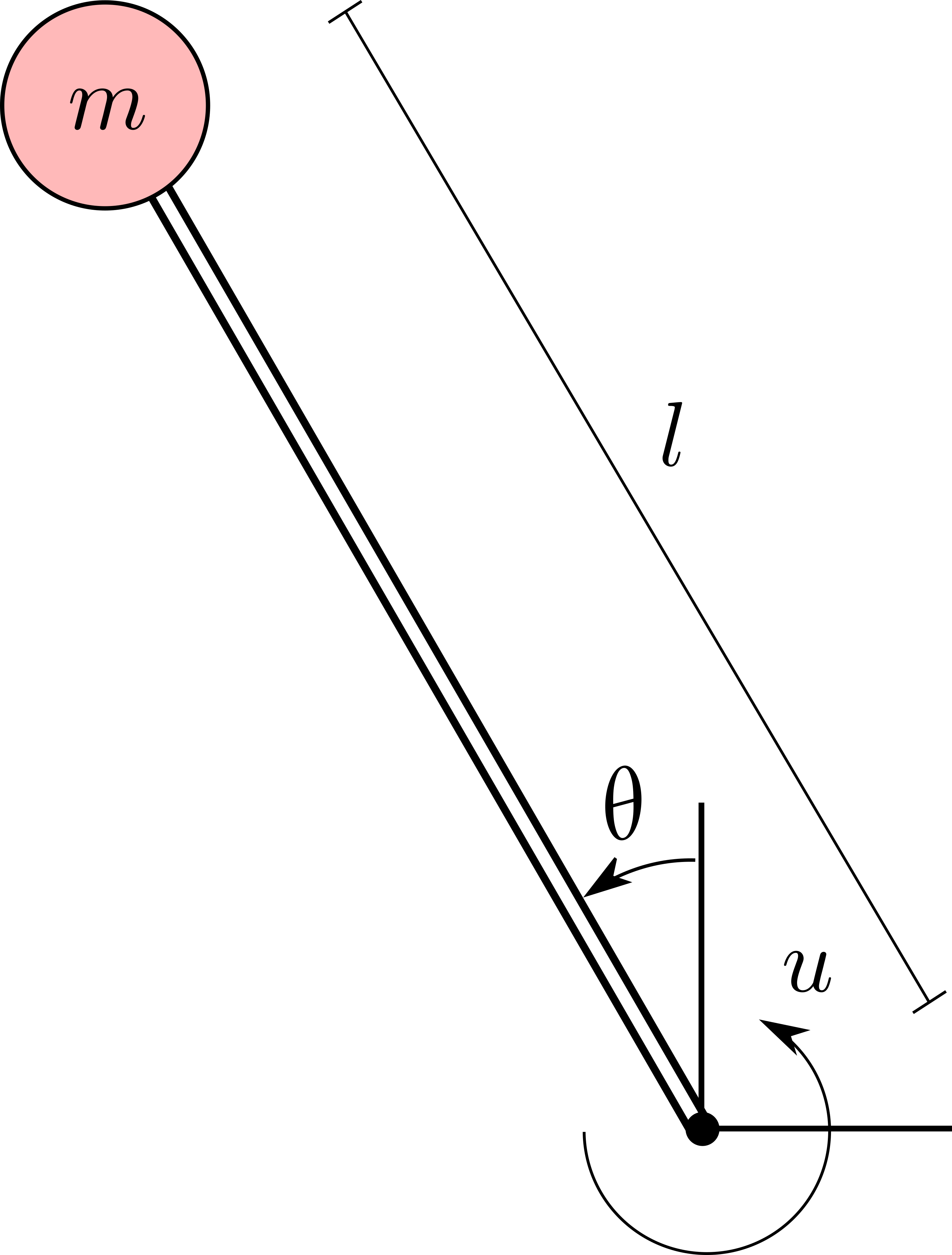
Consider the inverted pendulum shown in Figure 3.3. Its nonlinear dynamics are given by:

ml^{2}\ddot{\theta}=mgl\sin(\theta)+u,

where $m$ denotes the mass, $l$ is the length of the rod, $g$ is the acceleration due to gravity, $\theta$ is the pendulum angle, and $u$ is the control torque. Introducing the state vector $\bm{x}\coloneqq\left[{\theta\ \dot{\theta}}\right]^{\top}$ , the system can be written in state-space form as:

\dot{\bm{x}}=f(\bm{x},u)=\begin{bmatrix}\dot{\theta}\\ \frac{g}{l}\sin(\theta)+\frac{1}{ml^{2}}u\end{bmatrix}.

The upright stationary position $\bar{x}=\left[{0,0}\right]^{\top}$ is an equilibrium point for this system with equilibrium control input $\bar{u}=0$ . Linearizing about this equilibrium—one where $\delta\bm{x}=\bm{x}-\bar{\bm{x}}=\bm{x}$ and $\delta u=u-\bar{u}=u$ —yields the linear model:

\delta\dot{\bm{x}}=\begin{bmatrix}0&1\\ \frac{g}{l}&0\end{bmatrix}\delta\bm{x}+\begin{bmatrix}0\\ \frac{1}{ml^{2}}\end{bmatrix}\delta u,

whose state matrix has one eigenvalue with positive real part, and is therefore unstable.

To stabilize the pendulum, we can design a proportional–derivative controller of the form:

\delta u(t)=-k_{p}\theta(t)-k_{d}\dot{\theta}(t),

which would yield the closed-loop dynamics:

\delta\dot{\bm{x}}=\begin{bmatrix}0&1\\ \frac{g}{l}-\frac{1}{ml^{2}}k_{p}&-\frac{1}{ml^{2}}k_{d}\end{bmatrix}\delta\bm% {x}.

By selecting suitable gains $k_{p}>0$ and $k_{d}>0$ , we can ensure that both eigenvalues of the closed-loop system have negative real parts, ensuring stability around the upright position—analogously to the double-integrator PD design in Example 3.1.1. Of course, PD control is only one option, and other methods—such as the LQR—can also be applied to the linearized model.

Algorithm 3.3.1 shows a Python implementation of the linearization process for the inverted pendulum example using JAX, a library for high-performance numerical computing and automatic differentiation.

⬇

import jax

import jax.numpy as jnp

def inverted_pendulum_dynamics(x, u, g=9.81, m=1, l=1):

"""

Evaluate the inverted pendulum dynamics.

"""

\theta

, d

\theta

_dt = x

dx_dt = jnp.array([d

\theta

_dt, (g/l)*jnp.sin(

\theta

) + (1/m*l**2)*u])

return dx_dt

# Linearize around the stationary upright position with zero

# control (i.e. the pendulum is perfectly balanced)

f_jac = jax.jacobian(inverted_pendulum_dynamics, argnums=(0, 1))

x = jnp.array([0., 0.])

u = 0.

A, B = f_jac(x, u) # Evaluate Jacobian at equilibrium point

Algorithm 3.3.1: Linearizing the inverted pendulum dynamics from Example 3.3.1 in Python using the JAX library. The code for this example is available in the repository github.com/StanfordASL/pora-exercises in the notebook ch03/jax_linearization.ipynb.

3.3.3 Iterative LQR (iLQR) and Differential Dynamic Programming (DDP)

In the previous sections, we saw how the LQR framework—along with its various extensions—provides a principled foundation for regulation and tracking, and how the same ideas can be applied to both linear and nonlinear systems. Specifically, we highlighted how LQR can be naturally embedded within a two-step design paradigm, serving as a practical alternative to directly solving the full nonlinear optimal control problem by combining elements of open-loop trajectory generation and closed-loop tracking control.

In this section, we adopt a different yet complementary perspective, and explore how ideas from linearization and LQR can be extended to develop algorithms that simultaneously generate an open-loop trajectory and a closed-loop tracking controller in two-step design form. This approach leads to two closely related algorithms: the iterative linear quadratic regulator (iLQR) and differential dynamic programming (DDP). As we will see, the key insight underlying both methods is that the structure which makes LQR tractable—namely, quadratic cost and linear dynamics—can be embedded within an iterative optimization scheme to efficiently handle nonlinear dynamics and non-quadratic costs.

Iterative LQR.

Recall from the LQR tracking problem in Section 3.2.2 that the controller acts to drive deviation variables $(\delta\bm{x},\delta\bm{u})$ to zero, thereby ensuring the system follows a specified reference. At its core, iLQR uses the same machinery, but with a different objective: instead of driving the deviation variables to zero, the optimal deviations are used to modify the nominal trajectory itself. By repeating this process, iLQR gradually refines the trajectory until no further improvement can be made, yielding a locally optimal solution.

Formally, consider the discrete-time finite-horizon nonlinear optimal control problem:

\begin{split}\underset{[}{\text{minimize}}\>\quad\bm{u}]&h(\bm{x}_{N})+\sum_{t% =0}^{N-1}g(\bm{x}_{t},\bm{u}_{t}),\\ \text{subject to}\quad&\bm{x}_{t+1}=f(\bm{x}_{t},\bm{u}_{t}),\quad t=0,\ldots,% N-1,\\ \end{split}

(3.45)

Given a feasible nominal trajectory $(\bar{x}_{0},\bar{u}_{0},\ldots,\bar{x}_{N},\bar{u}_{N})$ , let us linearize the dynamics and quadratize the cost around the nominal trajectory as:

$\displaystyle\delta\bm{x}_{t+1}\approx$	$\displaystyle\underbrace{\frac{\partial f}{\partial x}\left(\bar{x}_{t},\bar{u% }_{t}\right)}_{\coloneqq A_{t}}\delta\bm{x}_{t}+\underbrace{\frac{\partial f}{% \partial u}\left(\bar{x}_{t},\bar{u}_{t}\right)}_{\coloneqq B_{t}}\delta\bm{u}% _{t}+\underbrace{0}_{\coloneqq c_{t}},$	(3.46)
$\displaystyle h(x_{N})\approx$	$\displaystyle\underbrace{h\left(\bar{x}_{N}\right)}_{\coloneqq\alpha_{f}}+% \underbrace{\nabla h\left(\bar{x}_{N}\right)}_{\coloneqq q_{f}}\delta\bm{x}_{N% }+\frac{1}{2}\delta\bm{x}_{N}\underbrace{\nabla^{2}h\left(\bar{x}_{N}\right)}_% {\coloneqq Q_{f}}\delta\bm{x}_{N},$
$\displaystyle g_{t}(x_{t},u_{t})\approx$	$\displaystyle\underbrace{g_{t}\left(\bar{x}_{t},\bar{u}_{t}\right)}_{\coloneqq% \alpha_{t}}+\underbrace{\nabla_{x}g\left(\bar{x}_{t},\bar{u}_{t}\right)}_{% \coloneqq q_{t}}\delta\bm{x}_{t}+\underbrace{\nabla_{u}g\left(\bar{x}_{t},\bar% {u}_{t}\right)}_{\coloneqq r_{t}}\delta\bm{u}_{t}$
	$\displaystyle+\frac{1}{2}\delta\bm{x}_{t}^{\top}\underbrace{\nabla_{xx}^{2}g_{% t}\left(\bar{x}_{t},\bar{u}_{t}\right)}_{\coloneqq Q_{t}}\delta\bm{x}_{t}+% \frac{1}{2}\delta\bm{u}_{t}^{\top}\underbrace{\nabla_{uu}^{2}g_{t}\left(\bar{x% }_{t},\bar{u}_{t}\right)}_{\coloneqq R_{t}}\delta\bm{u}_{t}$
	$\displaystyle+\delta\bm{x}_{t}^{\top}\underbrace{\nabla_{xu}^{2}g_{t}\left(% \bar{x}_{t},\bar{u}_{t}\right)}_{\coloneqq S_{t}}\delta\bm{u}_{t},$

where $Q, R, S$ are Hessians and $q, r$ the gradients of the cost with respect to state and input, evaluated along $(\bar{\bm{x}},\bar{\bm{u}})$ . This reduces the problem to the LQR formulation introduced in Equation 3.27, which can be solved via the Riccati equations to obtain the optimal deviations $(\delta\bm{x}^{*},\delta\bm{u}^{*})$ .

iLQR alternates between two complementary steps:

•

Backward pass: linearize the dynamics and quadratize the cost around $(\bar{\bm{x}},\bar{\bm{u}})$ . Solve the resulting LQR problem to obtain the affine control law for the deviation variables:

$\delta\bm{u}_{t}^{*}=-K_{t}\delta\bm{x}_{t}-k_{t}.$ (3.47)
•

Forward pass: starting from the initial condition $x_{0}$ , propagate the nonlinear system forward using:

$\bm{u}_{t}=\bar{\bm{u}}_{t}-k_{t}-K_{t}(\bm{x}_{t}-\bar{\bm{x}}_{t}),$ (3.48)

and update the nominal trajectory to $(\bar{\bm{x}},\bar{\bm{u}})=(\bm{x},\bm{u})$ .

These steps are repeated until the trajectory converges, typically measured by negligible improvement in cost or small changes in the control sequence.

Practical considerations.

While iLQR provides a powerful framework for trajectory optimization, its performance depends critically on several implementation details:

•

Local optimality. iLQR produces solutions that are only locally optimal. The resulting open-loop trajectory $(\bar{\bm{x}},\bar{\bm{u}})$ minimizes the cost only in a neighborhood of the initial guess, and the associated feedback law stabilizes the system only locally. Consequently, a good initialization of the nominal trajectory is often critical to success.
•

Second-order terms. The quadratic expansion of the cost introduces second-order terms $H_{xx,t}$ and $H_{uu,t}$ , which in general may not be positive semidefinite and positive definite, respectively. To ensure well-posed Riccati recursions, these terms are often regularized to be invertible, for example by adding a multiple of the identity matrix $(H_{xx,t}+\mu I$ , $H_{uu,t}+\mu I)$ , with $\mu>0$ , or by projecting them to the nearest valid matrices.
•

Termination criteria. Since iLQR is iterative, a stopping rule must be defined. In practice, iterations are terminated either when the change in the control trajectory is sufficiently small, or when the improvement in cost between successive iterations falls below a chosen threshold.
•

Forward pass robustness. During the forward pass, care must be taken to ensure that the updated trajectory does not deviate too far from the one used in the linearization. Common strategies include penalizing large deviations more heavily or performing a line search on the step size used to update the controls and states.

These considerations are critical for achieving robust and efficient performance in practice. A comprehensive collection of tips and detailed mathematical treatment of iLQR can be found in Tassa (2011)¹⁰10. Tassa, Y. Theory and Implementation of Biomimetic Motor Controllers. PhD Thesis. The Hebrew University of Jerusalem, 2011..

Differential dynamic programming.

Closely related to iLQR is DDP, an algorithm rooted in both LQR and dynamic programming^†^†margin: Introduced in Section 3.3.1 and which will be further discussed in the referenced item. . Like iLQR, DDP alternates between a backward pass (computing locally optimal gains) and a forward rollout (updating the trajectory). The key difference lies in the treatment of the backward pass. In iLQR, the dynamics are linearized to first order, so the resulting formulation involves second-order terms only from the cost function. In contrast, DDP also expands the dynamics to second order, so that curvature information from the nonlinear dynamics explicitly enters the Riccati recursion.

Formally, compared to the solution introduced in Equation 3.29, DDP augments the matrices $H_{xx,t}$ , $H_{uu,t}$ , and $H_{xu,t}$ with additional second-order terms, as follows:

$\displaystyle H_{xx,t}$	$\displaystyle\coloneqq Q_{t}+A_{t}^{\top}P_{t+1}A_{t}+\sum_{i=1}^{n}p_{t+1,i}% \,\nabla^{2}_{xx}f_{i}(\bar{\bm{x}}_{t},\bar{\bm{u}}_{t}),$	(3.49)
$\displaystyle H_{uu,t}$	$\displaystyle\coloneqq R_{t}+B_{t}^{\top}P_{t+1}B_{t}+\sum_{i=1}^{n}p_{t+1,i}% \,\nabla^{2}_{uu}f_{i}(\bar{\bm{x}}_{t},\bar{\bm{u}}_{t}),$
$\displaystyle H_{xu,t}$	$\displaystyle\coloneqq S_{t}+A_{t}^{\top}P_{t+1}B_{t}+\sum_{i=1}^{n}p_{t+1,i}% \,\nabla^{2}_{xu}f_{i}(\bar{\bm{x}}_{t},\bar{\bm{u}}_{t}).$

In practice, this richer approximation often improves convergence behavior and solution accuracy, especially in strongly nonlinear systems. However, it also makes DDP more computationally expensive than iLQR, since it requires evaluating and storing second-order derivatives of the dynamics at every iteration.

3.4 Model Predictive Control (MPC)

We now turn to Model Predictive Control (MPC), also known as Receding Horizon Control (RHC), which has become one of the most influential methodologies in modern control, both in theory and in practice. To appreciate its role, it is helpful to revisit the distinction between open-loop and closed-loop control.

In an open-loop formulation, the control problem is posed as finding a trajectory $\bm{u}(t)$ that optimizes a given performance criterion subject to system constraints. While conceptually straightforward and computationally cheaper, this approach does not account for disturbances or deviations from the nominal trajectory that may arise during execution.

By contrast, closed-loop control directly maps the measured state to a control action through a feedback policy. This design enables the control input to adapt to the current system state. However, computing optimal feedback policies can quickly become intractable, even for systems of moderate size^†^†margin: Earlier, we introduced PID controllers and LQR as computationally efficient examples of closed-loop control. These methods, however, are restricted to relatively simple settings such as linear systems with quadratic costs. More general cases often quickly become computationally prohibitive. .

At a high level, MPC can be seen as a principled unification of these two paradigms, using repeated open-loop optimization to effectively achieve closed-loop behavior. At each time step, MPC solves a finite-horizon open-loop optimal control problem, yielding an input sequence $u_{0},u_{1},\ldots,u_{N-1}$ . Only the first control action $u_{0}$ is applied, after which the horizon shifts forward, the state is re-measured, and the optimization is solved again. This receding-horizon strategy effectively embeds feedback into open-loop optimization, combining the robustness of closed-loop adaptation with the computational tractability of open-loop planning.

Naturally, MPC requires additional design elements to ensure reliable operation. Two key concerns are persistent feasibility (the guarantee that a valid solution can be found at each step) and stability (ensuring the closed-loop system behaves well over time). These are typically addressed through terminal constraints, tailored terminal costs, or other problem-specific design choices, which we will return to later in this section.

Historically, MPC emerged in the 1970s within the process control community, particularly in chemical engineering. This application domain was ideal for two reasons. First, safety-critical constraints (e.g., temperature limits) could be enforced explicitly within the optimization problem. Second, chemical processes evolve on relatively slow timescales, giving ample time to solve optimization problems online—even with the limited computational power of the era. With today’s hardware, these limitations have largely disappeared, and MPC is now deployed in real-time domains such as robotics, where numerical optimization problems may be solved at tens or hundreds of Hertz.

Today, MPC is considered one of the cornerstones of modern control. Alongside PID control and LQR, it is among the most widely applied methodologies, valued for its ability to explicitly handle constraints while maintaining robustness. The material in this section provides the foundations necessary to understand and implement MPC. For readers interested in deeper coverage of both theory and practice, we recommend the textbooks by Borrelli et al. (2017)¹¹11. Borrelli, F., Bemporad, A., Morari, M. Predictive Control for Linear and Hybrid Systems. Cambridge University Press, 2017. and Rawlings et al. (2017)¹²12. Rawlings, J., Mayne, D.Q., Diehl, M. Model Predictive Control: Theory, Computation, and Design. Nob Hill Publishing, 2017..

3.4.1 The Receding Horizon Framework

The underlying setting for MPC is the discrete-time infinite-horizon optimal control problem. That is, in principle, we would like to design a feedback policy that minimizes a cost accumulated over an infinite time horizon, that is, with final time $t_{f}=+\infty$ . Solving for closed-loop policies in this setting is, however, typically intractable.

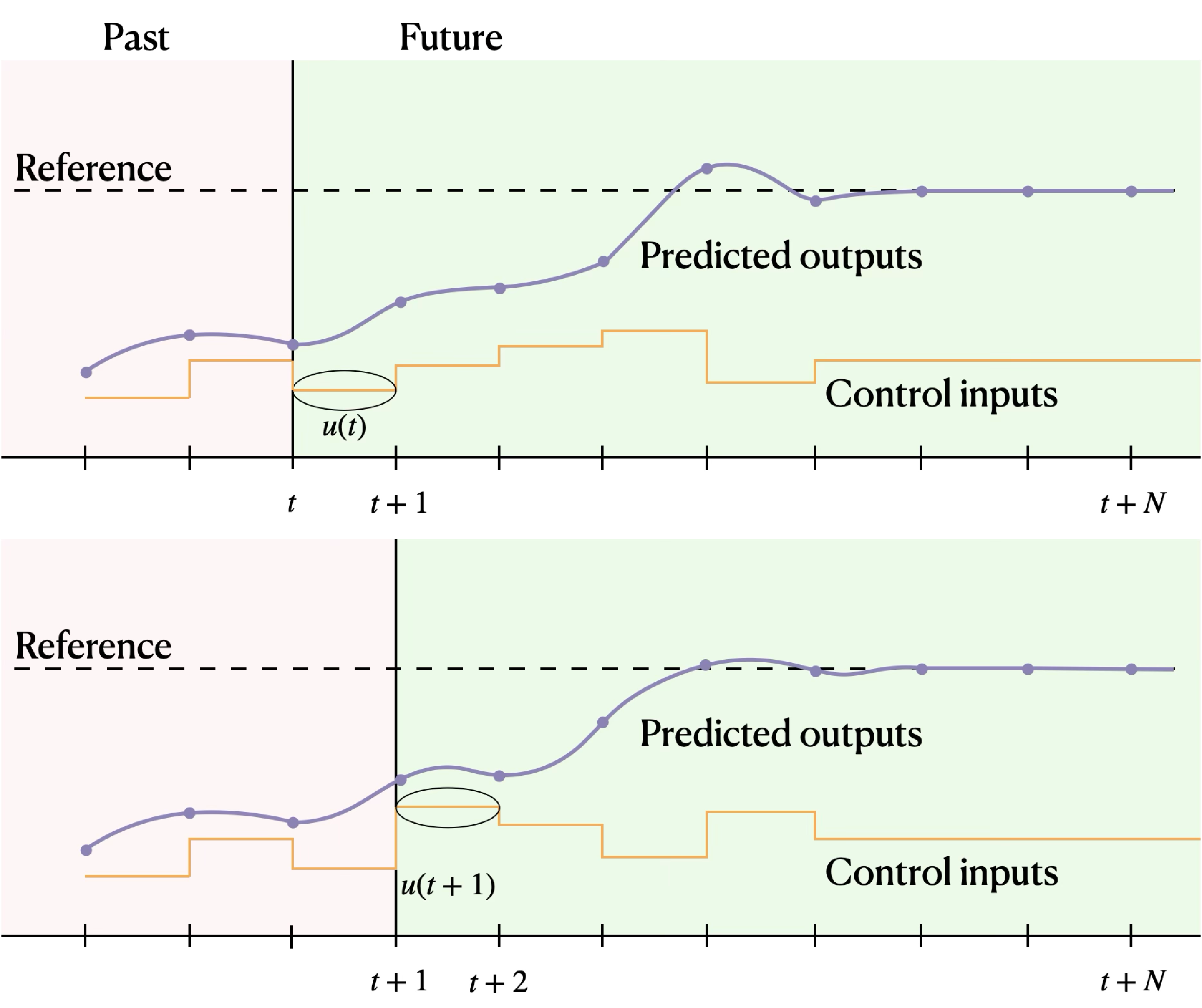
MPC addresses this challenge through a suboptimal—but computationally tractable—approximation. Essentially, instead of solving the infinite-horizon problem directly, it repeatedly solves a finite-horizon optimal control problem. The idea is simple and illustrated in Figure 3.4. At the current time $t$ , the system state is measured, and an optimal control sequence is computed over a horizon of length $N$ . As in any open-loop formulation, the optimization relies on the system model to predict how the state will evolve under candidate input sequences, selecting the one that minimizes the cost over the finite horizon. This process yields a sequence of control inputs:

u_{t},u_{t+1},\ldots,u_{t+N-1},

along with the corresponding predicted state trajectory. Crucially, only the first control input $u_{t}$ is applied to the system. Once time advances to $t+1$ , the remaining inputs $u_{t+1},\ldots,u_{t+N-1}$ are discarded, and a new optimization problem is solved based on the updated state measurement. This process is then repeated recursively.

This scheme is often referred to as the receding horizon framework, where the horizon “moves forward” with time, and at each step a new optimization problem is solved based on the latest state information. While it may appear wasteful to discard the unused portion of the control trajectory, this is precisely what allows MPC to incorporate updated measurements and disturbances, ensuring feedback is embedded into the process.

If the finite-horizon problems are designed and tuned carefully—through appropriate horizon lengths, terminal costs, or constraints—the closed-loop behavior of MPC can closely approximate that of the true infinite-horizon optimal controller. In practice, MPC often achieves performance nearly indistinguishable from the infinite-horizon optimal solution, while remaining computationally feasible.

3.4.2 Basic Formulation

To formalize the ideas introduced above, consider the discrete-time linear time-invariant (LTI) system:

\bm{x}_{t+1}=A\bm{x}_{t}+B\bm{u}_{t},

(3.50)

where $\bm{x}_{t}\in\mathbb{R}^{n}$ and $\bm{u}_{t}\in\mathbb{R}^{m}$ denote the state and input vectors, respectively. Both are subject to constraints of the form:

\bm{x}_{t}\in\mathcal{X},\quad\bm{u}_{t}\in\mathcal{U},\quad\forall t\geq 0,

(3.51)

where $\mathcal{X}\subseteq\mathbb{R}^{n}$ and $\mathcal{U}\subseteq\mathbb{R}^{m}$ are convex polyhedral sets describing admissible states and inputs.

At time $t$ , given the measured state $\bm{x}_{t}$ , MPC computes an input sequence over a prediction horizon of length $N$ :

\bm{u}_{t|t},\,\bm{u}_{t+1|t},\,\dots,\,\bm{u}_{t+N-1|t},

where the notation $\bm{u}_{t+k|t}$ indicates “the input applied at time $t+k$ as predicted at time $t$ ”. Correspondingly, we denote the predicted state trajectory as:

\bm{x}_{t|t},\,\bm{x}_{t+1|t},\,\dots,\,\bm{x}_{t+N|t},\qquad\text{with }\bm{x% }_{t|t}=\bm{x}_{t}.

Finite-horizon problem.

The control inputs are obtained by solving the finite-horizon optimal control problem:

$\displaystyle J_{t}^{*}(\bm{x}_{t})=\underset{[}{\text{minimize}}\>\quad% \mathcal{U}_{t\to t+N\|t}]$	$\displaystyle h(\bm{x}_{t+N\|t})+\sum_{k=0}^{N-1}g(\bm{x}_{t+k\|t},\bm{u}_{t+k\|t% }),$	(3.52)
subject to	$\displaystyle\bm{x}_{t+k+1\|t}=A\bm{x}_{t+k\|t}+B\bm{u}_{t+k\|t},\quad k=0,\dots,% N-1,$
	$\displaystyle\bm{x}_{t+k\|t}\in\mathcal{X},\ \bm{u}_{t+k\|t}\in\mathcal{U},\quad k% =0,\dots,N-1,$
	$\displaystyle\bm{x}_{t+N\|t}\in\mathcal{X}_{f},\quad\bm{x}_{t\|t}=\bm{x}_{t},$

where $\mathcal{U}_{t\to t+N|t}$ denotes the sequence of decision variables ${\bm{u}_{t|t},\dots,\bm{u}_{t+N-1|t}}$ , $\mathcal{X}_{f}$ is a terminal set, and the functions $g(\cdot,\cdot)$ and $h(\cdot)$ represent stage and terminal costs.

Control law.

Only the first element of the optimal input sequence is applied to the system:

\bm{u}_{t}=\bm{u}_{t|t}^{*}(\bm{x}_{t}),

(3.53)

where the dependency on $\bm{x}_{t}$ arises from the fact that the optimization problem in Equation 3.52 has the condition $\bm{x}_{t|t}=\bm{x}_{t}$ . At the next step, $t+1$ , the state is re-measured, and Problem (Equation 3.52) is solved again with updated information. This iterative procedure defines the receding horizon control law, embedding feedback into the overall process.

Closed-loop dynamics.

The resulting closed-loop system can be written compactly as:

\bm{x}_{t+1}=A\bm{x}_{t}+B\pi_{t}(\bm{x}_{t})=f_{\mathrm{cl}}(\bm{x}_{t}),% \qquad t\geq 0,

(3.54)

where $\pi_{t}(\bm{x}_{t})\coloneqq\bm{u}_{t|t}^{*}(\bm{x}_{t})$ is the MPC feedback law at time $t$ . Because the dynamics, cost, and constraints are time-invariant, the problem can be equivalently written by fixing the initial time $t=0$ . Formally, let $\bm{x}_{0}=\bm{x}_{t}$ and $\mathcal{U}_{0}={\bm{u}_{0},\dots,\bm{u}_{N-1}}$ , we can rewrite the problem in Equation 3.52 as:

$\displaystyle J_{0}^{*}(\bm{x}_{t})=\underset{[}{\text{minimize}}\>\quad% \mathcal{U}_{0}]$	$\displaystyle h(\bm{x}_{N})+\sum_{k=0}^{N-1}g(\bm{x}_{k},\bm{u}_{k}),$	(3.55)
subject to	$\displaystyle\bm{x}_{k+1}=A\bm{x}_{k}+B\bm{u}_{k},\quad k=0,\dots,N-1,$
	$\displaystyle\bm{x}_{k}\in\mathcal{X},\ \bm{u}_{k}\in\mathcal{U},\quad k=0,% \dots,N-1,$
	$\displaystyle\bm{x}_{N}\in\mathcal{X}_{f},\quad\bm{x}_{0}=\bm{x}_{t}.$

This formulation is often more convenient for analysis, since it avoids carrying the explicit time index through the condition $\bm{x}_{0}=\bm{x}_{t}$ .

Typical cost functions.

In practice, MPC problems are often defined by quadratic stage and terminal costs of the form:

h(\bm{x}_{N})=\bm{x}_{N}^{\top}Q_{f}\bm{x}_{N},\qquad g(\bm{x}_{k},\bm{u}_{k})% =\bm{x}_{k}^{\top}Q\bm{x}_{k}+\bm{u}_{k}^{\top}R\bm{u}_{k},

(3.56)

with $Q_{f}\succeq 0$ , $Q\succeq 0$ , and $R\succ 0$ . This leads to the overall cost function:

J_{0}(\bm{x}_{0})=\bm{x}_{N}^{\top}Q_{f}\bm{x}_{N}+\sum_{k=0}^{N-1}\big{(}\bm{% x}_{k}^{\top}Q\bm{x}_{k}+\bm{u}_{k}^{\top}R\bm{u}_{k}\big{)}.

(3.57)

Quadratic costs are not only natural but also lead to convex optimization problems when paired with polyhedral constraints. Alternative norms, such as $\ell_{1}$ or $\ell_{\infty}$ , are sometimes used to promote robustness or sparsity in the control actions^†^†margin: For instance, $\ell_{1}$ penalties are commonly used in predictive control formulations for systems with actuator limitations or to induce sparse actuation. .

Implementation challenges.

While MPC provides a powerful framework, it also raises two critical implementation challenges:

1.

Persistent feasibility. Even if the optimization problem is feasible at the current time step, there is no guarantee that feasibility will be preserved in the future, as the chosen inputs may drive the system into a region of the state space from which no admissible solution exists. This situation arises when the controller fails to “look ahead” sufficiently to maintain long-term feasibility. For example, consider an autonomous car driving towards an obstacle at high speed, and the MPC controller chooses to brake too late because of a short-sighted horizon. As a result, the car may end up in a state where it cannot stop in time to avoid a collision, leading to infeasibility in subsequent control steps.
2.

Closed-loop stability. Feasibility alone does not guarantee that the closed-loop trajectories converge to the origin. In fact, it is possible for the MPC law to produce admissible control inputs that indefinitely satisfy the constraints but fail to stabilize the system.

These issues highlight a fundamental tension: MPC is based on solving short-horizon problems, yet we ultimately require effective long-term behavior. How can a strategy that looks only $N$ steps ahead ensure both feasibility and stability over a potentially infinite horizon?

A central insight is that these properties can be enforced through appropriate design of the terminal cost and terminal constraint set—denoted as $h(\cdot)$ and $\mathcal{X}_{f}$ in (Equation 3.52), respectively. Roughly speaking, the terminal cost serves as a surrogate for the infinite-horizon tail of the problem, while the terminal set ensures that the system remains within a region where the behavior is well-understood and manageable. Together, these design choices represent a flexible tool to reconcile the short-sighted nature of MPC with the long-term guarantees we ultimately care about.

While a full treatment of these issues is beyond the scope of this book, we refer the interested reader to Borrelli et al. (2017)¹³13. Borrelli, F., Bemporad, A., Morari, M. Predictive Control for Linear and Hybrid Systems. Cambridge University Press, 2017. for comprehensive discussions and rigorous treatments of these topics.

3.4.3 MPC for Tracking: Delta Input $(\delta\bm{u})$ Formulation

A particularly common use case for MPC is reference tracking, where the objective is to have the system state follow a reference trajectory $\bm{r}_{0},\bm{r}_{1},\ldots$ over time. Here, $\bm{r}_{t}\in\mathbb{R}^{p}$ may denote the full state reference (in which case $p=n$ ) or a partial output reference (with $p<n$ ). In this section, we introduce the $\delta\bm{u}$ formulation¹⁸18. Borrelli, F., Bemporad, A., Morari, M. Predictive Control for Linear and Hybrid Systems. Cambridge University Press, 2017. which is particularly advantageous in trajectory tracking and regulation tasks around nonzero operating points.

Formally, consider the following LTI system:

\begin{split}\bm{x}_{t+1}&=A\bm{x}_{t}+B\bm{u}_{t},\\ \bm{u}_{t}&=\bm{u}_{t-1}+\delta\bm{u}_{t},\\ \bm{y}_{t}&=C\bm{x}_{t},\end{split}

(3.58)

where $\delta\bm{u}_{t}\in\mathbb{R}^{m}$ represents the change in control input from the previous time step, $\bm{y}_{t}\in\mathbb{R}^{p}$ denotes the system output at time $t$ , and $C\in\mathbb{R}^{p\times n}$ is a linear transformation mapping the state to the output. Assuming the pair $(A,B)$ is controllable, it is often desirable to parameterize the optimization problem in terms of the control increments rather than the absolute control inputs. Instead of optimizing the inputs $\bm{u}_{t},\bm{u}_{t+1},\ldots,\bm{u}_{t+N-1}$ directly, the controller optimizes their increments:

\delta\bm{u}_{t}=\bm{u}_{t}-\bm{u}_{t-1},

(3.59)

and reconstructs the actual inputs recursively as:

\bm{u}_{t}=\bm{u}_{t-1}+\delta\bm{u}_{t},

(3.60)

with the idea that, once the system has reached a steady state, the control inputs will remain constant (that is, $\delta\bm{u}_{t}=0$ ).

As a result, the MPC problem can be readily reformulated as:

$\displaystyle J_{0}^{*}(\bm{x}_{t})=\underset{[}{\text{minimize}}\>\quad\delta% \bm{u}_{0},\ldots,\delta\bm{u}_{N-1}]$	$\displaystyle\sum_{k=0}^{N-1}y_{k}^{\top}Q\bar{x}_{k}+\delta u_{k}^{\top}R% \delta u_{k},$	(3.61)
subject to	$\displaystyle\bm{x}_{k+1}=A\bm{x}_{k}+B\bm{u}_{k},\quad k=0,\dots,N-1,$
	$\displaystyle y_{k}=C\bm{x}_{k},\quad k=0,\dots,N-1,$
	$\displaystyle\bm{x}_{k}\in\mathcal{X},\quad\bm{u}_{k}\in\mathcal{U},\quad k=0,% \dots,N-1,$
	$\displaystyle\bm{x}_{N}\in\mathcal{X}_{f},$
	$\displaystyle\bm{u}_{k}=\bm{u}_{k-1}+\delta\bm{u}_{k},\quad k=0,\dots,N-1,$
	$\displaystyle\bm{x}_{0}=\bm{x}(t),\quad\bm{u}_{-1}=\bm{u}(t-1),$

where $\bm{x}(t)$ and $\bm{u}(t-1)$ denote the current state and the last applied control input, respectively.

Ultimately, the $\delta\bm{u}$ formulation does not change the fundamental structure of MPC but reparameterizes the optimization problem in a way that is better conditioned for tracking tasks.

3.4.4 Receding Horizon as a General Principle for Real-World Control

In practice, virtually all implementations of optimal control—whether framed as MPC, closed-loop form, or as a two-step design—operate according to the receding horizon framework. Even when a nominal trajectory is first computed offline and subsequently tracked by a feedback controller, the controller is typically reinitialized and re-optimized as new state information becomes available. In other words, the nominal trajectory serves only as a temporary reference, continuously adjusted as the system evolves and new measurements are obtained. This viewpoint helps reconcile the apparent distinction between MPC and trajectory-tracking control: both ultimately rely on repeated, finite-horizon optimization combined with feedback, differing mainly in how frequently and to what extent the optimization is repeated. Recognizing this continuity is important, as it clarifies that the so-called “receding horizon” behavior is not unique to MPC, but rather a practical necessity in virtually all control architectures that seek robustness to uncertainty and disturbances.

3.5 Summary

In this chapter, we introduced strategies for closed-loop control and trajectory tracking. Specifically, we discussed how the goal of closed-loop control is to compute a control policy that continuously adapts to the system’s evolving state. While generally more computationally demanding than open-loop methods, closed-loop control provides substantial advantages in terms of robustness to disturbances, model inaccuracies, and external perturbations.

We also introduced a tractable compromise through the concept of a two-step design, in which an open-loop trajectory is first computed and then tracked using a feedback controller. This formulation allowed us to naturally transition to trajectory-tracking control, bridging open-loop optimization and closed-loop stabilization.

Building on these concepts, the chapter presented several key methods for closed-loop control and trajectory tracking. We began with classical feedback control, illustrated by the PID controller and its application to trajectory tracking, particularly for differentially flat systems. We then introduced linear optimal control methods, focusing on the linear quadratic regulator, which provides an elegant closed-form solution for linear systems via the Riccati equation and extends naturally to tracking problems.

Next, we turned to nonlinear optimal control. We first contextualized techniques for obtaining globally optimal closed-loop solutions—namely dynamic programming and the HJB equation—and then showed how the notion of linearization enables the use of LQR for local stabilization and trajectory tracking in nonlinear systems. Building on this, we discussed how algorithms such as iLQR and DDP extend these principles to simultaneously generate an open-loop trajectory and a closed-loop tracking controller in two-step design form.

Finally, we presented model predictive control as a powerful framework that unifies open-loop optimization with closed-loop feedback through a receding-horizon strategy, offering a versatile method for handling constraints in real-time applications.

To learn more.

For a deeper exploration of the topics covered in this chapter, several key resources are available. An in-depth treatment of feedback control and PID controllers can be found in Aström and Murray (2009)¹⁴14. Aström, K. J., Murray, R. M. Feedback Systems. Princeton University Press, 2009.. For a rigorous treatment of optimal control from a dynamic programming perspective, which provides the theoretical underpinnings for the Riccati equation, Bertsekas (2000)¹⁵15. Bertsekas, D. Dynamic Programming and Optimal Control. Athena Scientific, 2000. is an essential reference. Finally, for comprehensive coverage of model predictive control, from fundamental principles to advanced theory and applications, we refer the reader to the textbooks by Rawlings et al. (2017)¹⁶16. Rawlings, J., Mayne, D.Q., Diehl, M. Model Predictive Control: Theory, Computation, and Design. Nob Hill Publishing, 2017. and Borrelli et al. (2017)¹⁷17. Borrelli, F., Bemporad, A., Morari, M. Predictive Control for Linear and Hybrid Systems. Cambridge University Press, 2017..

3.6 Exercises

The starter code for the exercises provided below is available online through GitHub. To get started, download the code by running in a terminal window:

⬇

git clone https://github.com/StanfordASL/pora-exercises.git

We denote Problems requiring hand-written solutions and coding in Python with and , respectively.

Problem 1: Inverted Pendulum PD Control

In the notebook ch03/exercises/pid_control.ipynb, implement the PD controller for the inverted pendulum dynamics. Then, play around with different values of the gains $k_{p}$ and $k_{d}$ and use JAX and NumPy to compute the Jacobian of the closed-loop dynamics. Verify the eigenvalues of the linearized matrix are stable. Finally, run the provided code to simulate the nonlinear closed-loop dynamics.

Problem 2: Cart-pole LQR Control

In this problem, we consider a cart-pole formulation in which we will design a controller to balance an inverted pendulum by linearizing the dynamics around a single stationary point. Therefore, we will consider a trajectory initialized in a neighborhood about the final, upright state and the optimal control is a closed-form solution derived through Riccati recursion. This system has two degrees of freedom corresponding to the horizontal position $x$ of the cart, and the angle $\theta$ of the pendulum (where $\theta=0$ occurs when the pendulum is hanging straight downwards). We can apply a force $u\in\mathbb{R}$ to push the cart horizontally, where $u>0$ corresponds to a force in the positive $x$ -direction. With the state $s\coloneqq(x,\theta,\dot{x},\dot{\theta})\in\mathbb{R}^{4}$ , we can write the continuous-time dynamics of the cart-pole system as:

\dot{s}=f(s,u)=\begin{bmatrix}\dot{x}\\ \dot{\theta}\\ \frac{m_{p}(\ell\dot{\theta}^{2}+g\cos\theta)\sin\theta+u}{m_{c}+m_{p}\sin^{2}% \theta}\\[5.0pt] -\frac{(m_{c}+m_{p})g\sin\theta+m_{p}\ell\dot{\theta}^{2}\sin\theta\cos\theta+% u\cos\theta}{\ell(m_{c}+m_{p}\sin^{2}\theta)}\end{bmatrix},

where $m_{p}$ is the mass of the pendulum, $m_{c}$ is the mass of the cart, $\ell$ is the length of the pendulum, and $g$ is the acceleration due to gravity. We can discretize the continuous-time dynamics using Euler integration with a fixed time step $\Delta{t}$ to get the approximate discrete-time dynamics:

s_{k+1}\approx s_{k}+\Delta{t}f(s_{k},u_{k}),

where $s_{k}$ and $u_{k}$ are the state and control input, respectively, at time $t=k\Delta{t}$ . The code for this exercise is located in
ch03/exercises/cartpole_lqr_control.ipynb.

1.

Consider the upright state $\bar{s}\coloneqq(0,\pi,0,0)$ with $\bar{u}\coloneqq 0$ , and define $\tilde{s}_{k}\coloneqq s_{k}-\bar{s}$ . Linearizing the approximate discrete-time dynamics $s_{k+1}\approx s_{k}+\Delta{t}f(s_{k},u_{k})$ about $(\bar{s},\bar{u})$ yields an approximate LTI system of the form:

$\tilde{s}_{k+1}\approx A\tilde{s}_{k}+Bu_{k}.$

Express $A$ and $B$ in terms of $m_{p}$ , $m_{c}$ , $\ell$ , $g$ , and $\Delta{t}$ . You may use the fact that:

$\frac{\partial f}{\partial s}(\bar{s},\bar{u})=\begin{bmatrix}0&0&1&0\\ 0&0&0&1\\ 0&\frac{m_{p}g}{m_{c}}&0&0\\ 0&\frac{(m_{c}+m_{p})g}{m_{c}\ell}&0&0\end{bmatrix},\quad\frac{\partial f}{% \partial u}(\bar{s},\bar{u})=\begin{bmatrix}0\\ 0\\ \frac{1}{m_{c}}\\ \frac{1}{m_{c}\ell}\end{bmatrix}.$

We will design a stabilizing LQR controller for this discrete-time LTI system to solve:

	$\displaystyle\underset{[}{\text{minimize}}\>\quad u]{}$	$\displaystyle\sum_{k=0}^{\infty}\left(\frac{1}{2}\tilde{s}_{k}^{\mathsf{T}}Q% \tilde{s}_{k}+\frac{1}{2}u_{k}^{\mathsf{T}}Ru_{k}\right),$
	subject to	$\displaystyle\tilde{s}_{k+1}=A\tilde{s}_{k}+Bu_{k},\ \forall k\in\mathbb{N}_{% \geq 0},$

for fixed $Q,R\succ 0$ . Recall that after $N$ iterations of the discrete-time Riccati recursion:

	$\displaystyle K_{k}$	$\displaystyle=-(R+B^{\mathsf{T}}P_{k+1}B)^{-1}B^{\mathsf{T}}P_{k+1}A,$
	$\displaystyle P_{k}$	$\displaystyle=Q+A^{\mathsf{T}}P_{k+1}(A+BK_{k}),$

the cost-to-go matrices $\{P_{k}\}_{k=0}^{N}$ and the time-varying feedback gains $\{K_{k}\}_{k=0}^{N-1}$ describe the optimal LQR controller for a finite-horizon version of the problem above. If $(A,B)$ is stabilizable, then these iterates asymptotically converge to some $P_{\infty}\succ 0$ and $K_{\infty}$ . In fact, $J^{*}(s_{0})\coloneqq(s_{0}-\bar{s})^{\mathsf{T}}P_{\infty}{(s_{0}-\bar{s})}$ is the infinite-horizon optimal cost-to-go for any initialization $s_{0}$ , and $u_{k}=K_{\infty}\tilde{s}_{k}$ is the optimal feedback policy, which happens to be linear and time-invariant¹¹1 The infinite-horizon LQR problem also converges for fixed $Q\succeq 0$ and $R\succ 0$ , as long as $(A,B)$ is stabilizable and $(A,Q)$ is detectable. .

2.

Write code to approximate $P_{\infty}$ and $K_{\infty}$ for the linearized, discretized cart-pole system by initializing $P_{\infty}=0$ and then applying the Riccati recursion until convergence with respect to the maximum element-wise norm condition $\lVert P_{k}-P_{k-1}\rVert_{\mathrm{max}}<10^{-4}$ . Use $m_{p}=2~{}\mathrm{kg}$ , $m_{c}=10~{}\mathrm{kg}$ , $\ell=1~{}\mathrm{m}$ , $g=9.81~{}\mathrm{m/s}^{2}$ , $\Delta{t}=0.1~{}\mathrm{s}$ , $Q=I_{4}$ , and $R=I_{1}$ . Report the value of $K_{\infty}$ with two decimal places for each entry.
3.

Use the provided code to simulate the continuous-time, nonlinear cart-pole system with the linear feedback controller $u=K_{\infty}\tilde{s}$ . Initialize the system at $s=(0,3\pi/4,0,0)$ , and use a controller sampling rate of $10~{}\mathrm{Hz}$ . Verify from the simulation output that the behavior stabilizes as expected.
4.
We will now use an LQR controller to track a time-varying trajectory. Specifically, we will aim to balance the pendulum upright (that is, $\bar{\theta}(t)\equiv\pi$ ) while oscillating the position of the cart to track a desired reference $\bar{x}(t)=a\sin(2\pi t/T)$ , where $a>0$ and $T>0$ are known constants.
1. (a)
  
  Normally, as discussed in this chapter, you would have to re-linearize the system around the desired trajectory at each time step. Why is this not the case for this particular problem (that is, why can you just reuse $A$ and $B$ )?
2. (b)
  
  Repeat part (c) for this case with $a=10$ and $T=10$ , except this time initialize the system upright at $s(0)=(0,\pi,0,0)$ . For each state plot, overlay the corresponding entry from the reference trajectory $\bar{s}(t)$ .
3. (c)
  
  You may notice that this controller does not have good tracking performance. You could try increasing the state penalty matrix $Q$ to, e.g., $Q=10I_{4}$ . However, this should only improve tracking for $x(t)$ and $\dot{x}(t)$ , while $\theta(t)$ and $\dot{\theta}(t)$ still oscillate around $\pi$ and $0$ , respectively. What physical characteristic of the desired trajectory (or lack thereof) causes this to happen?

Problem 3: Cart-pole Swing Up (iLQR)

In this problem, we will implement a controller to solve the cart-pole “swing up” problem and will assume that we do not have actuation constraints. In the swing-up problem, the pendulum begins hanging downwards and is then brought to the upright position. Unlike in the cart-pole balancing problem, it is no longer sufficient to linearize around a single stationary point. Therefore, we will formulate the optimal control problem into a convex sub-problem and iteratively solve for optimal perturbations from a reference trajectory. Since we do not consider the case with limited actuation capabilities, the solution to each convex sub-problem can be solved with Riccati recursion, i.e., we will iteratively develop our solution using iterative LQR (iLQR) control. In this case, iLQR control provides an elegant and easy to implement closed-loop policy. However, through the standard LQR formulation at each iteration, we generally cannot reason, at least directly, over constraints on the state or control space: in the case of limited actuation, we require the more flexible and sophisticated framework provided by Sequential Convex Programming. The code for this exercise is located in ch03/exercises/cartpole_iterative_lqr.ipynb.

Recall that the cart-pole is a continuous-time system with dynamics of the form $\dot{s}=f(s,u)$ . To compute the iLQR control law, we will consider the Euler discretized dynamics:

s_{k+1}\approx f(s_{k},u_{k})\coloneqq s_{k}+\Delta{t}f(s_{k},u_{k}),

(3.62)

with time step $\Delta{t}>0$ . The provided code will then simulate this control law on the original continuous-time system.

1.

For a given operating point $(\bar{s}_{k},\bar{u}_{k})$ , suppose we define the Jacobians:

$A_{k}\coloneqq\frac{\partial f}{\partial s}(\bar{s}_{k},\bar{u}_{k}),\quad B_{% k}\coloneqq\frac{\partial f}{\partial u}(\bar{s}_{k},\bar{u}_{k}).$ (3.63)

Use JAX in the function linearize to write a single line of code that computes $A_{k}$ and $B_{k}$ , given $f$ , $\bar{s}_{k}$ and $\bar{u}_{k}$ .

For our iLQR controller, we will use the quadratic cost function:

J(s,u)\coloneqq\frac{1}{2}(s_{N}-s_{\mathrm{goal}})^{\mathsf{T}}Q_{N}(s_{N}-s_% {\mathrm{goal}})+\frac{1}{2}\sum_{k=0}^{N-1}\left((s_{k}-s_{\mathrm{goal}})^{% \mathsf{T}}Q(s_{k}-s_{\mathrm{goal}})+u_{k}^{\mathsf{T}}Ru_{k}\right),

(3.64)

where $s_{\mathrm{goal}}$ is the goal state (i.e., the upright position). The entries of $Q_{N}\succ 0$ are chosen to be large so that the terminal cost acts as a soft terminal “constraint”.

2.

Rewrite the cost function in terms of the deviations $\tilde{s}_{N}\coloneqq s_{N}-\bar{s}_{N}$ , $\tilde{s}_{k}\coloneqq s_{k}-\bar{s}_{k}$ , and $\tilde{u}_{k}\coloneqq u_{k}-\bar{u}_{k}$ . This will result in a quadratic cost function with linear terms of the form $q_{N}^{\mathsf{T}}\tilde{s}_{N}$ , $q_{k}^{\mathsf{T}}\tilde{s}_{k}$ , and $r_{k}^{\mathsf{T}}\tilde{u}_{k}$ . Identify the vectors $q_{N}$ , $q_{k}$ , and $r_{k}$ .
3.

Complete the iLQR controller code in the function
discreteIterativeLQR.solve. Specifically, your code must update the controller gain and offset terms $\{Y_{k}\}_{k=0}^{N-1}$ and $\{y_{k}\}_{k=0}^{N-1}$ , respectively²²2 In Section 3.3.3, we labeled these terms as $K_{t}$ and $k_{t}$ , but here we try to avoid confusion with the discrete index $k$ . , the nominal trajectory $(\bar{s},\bar{u})$ , and the deviations $(\tilde{s},\tilde{u})$ .
4.

Implement the function compute_control for the discreteIterativeLQR class to apply either the open-loop iLQR control input or the closed-loop iLQR policy, depending on the value of the Boolean flag closed_loop. Run your code for both cases to simulate the system and generate plots of the state and control input over time. You should notice that the iLQR control sequence does not accomplish the task if applied open-loop.

Problem 4: Linear MPC

In Section 3.4, we introduced some of the fundamental aspects of model predictive control. For this exercise, you will implement a simple MPC scheme for a linear system to drive the system to the origin while minimizing the cost function:

J(\bm{x}_{0})=\sum_{t=0}^{\infty}\big{(}\bm{x}_{t}^{\top}Q\bm{x}_{t}+\bm{u}_{t% }^{\top}R\bm{u}_{t}\big{)},

and satisfying the inequality constraints on the state and control, $\bm{x}_{t}\leq\bm{x}_{u}$ , $\bm{x}_{t}\geq\bm{x}_{l}$ , and $\lVert\bm{u}_{t}\rVert_{\infty}\leq r_{u}$ . To solve this problem with a finite-horizon MPC scheme, we will use the cost function from Equation 3.57 which adds a terminal cost and we will also add a terminal constraint $\lVert\bm{x}_{N}\rVert_{\infty}\leq r_{N}$ to the problem. In the notebook ch03/exercises/linear_mpc.ipynb:

1.

Implement the function solve_mpc to solve a finite horizon MPC problem with the quadratic stage and terminal costs, inequality constraints on the state and control, and the terminal constraint discussed above.
2.

Run the provided code to simulate the closed-loop system with the terminal cost $Q_{f}=Q$ and with no terminal constraint (that is, set $r_{N}=\infty$ ). Analyze the resulting plots, explain why there is a difference between the trajectory computed in each MPC iteration’s optimization problem and the final closed-loop trajectory.
3.

Next, run the provided code that specifies a different terminal cost matrix $Q_{f}$ by the solution to the discrete-time algebraic Riccati equation (DARE) from Equation 3.22 in the section on the linear quadratic regulator. What do you notice about the difference between the MPC trajectory computed at each time step and the closed-loop system behavior? Why is this different than when using $Q_{f}=Q$ ? Notice that the total cost of the closed-loop trajectory is lower when using the DARE terminal cost matrix, why is that?
4.

As we discussed in Section 3.4, persistent feasibility is a challenge with MPC, where we want to guarantee that if we find a feasible solution at one time step then we will be able to find a feasible solution at future time steps. One simple solution to this problem is to apply a terminal constraint $\bm{x}_{N}=0$ , which forces the optimizer to find a trajectory to the origin by the end of the finite horizon, thereby eliminating the issue with being short-sighted. However, this will cause the controller to be sub-optimal and can require a longer horizon to find a feasible solution. Run the provided code and play around with the controller’s horizon, how does the closed-loop trajectory’s cost change as the horizon changes?

Problem 5: Extended Unicycle Trajectory Tracking Control

In Example 3.1.2, we introduced a closed-loop trajectory tracking problem for a dynamically extended unicycle model where we apply a PD controller. In this example, we showed that since the system is differentially flat we could write its dynamics as the second order linear system in Equation 3.6. From these dynamics, we can develop a PD controller for the virtual inputs $w_{1}$ and $w_{2}$ given by Equation 3.7, and then can map these virtual controls back into the actual controls $(a,\omega)$ algebraically using:

\begin{bmatrix}a\\[3.0pt] \omega\end{bmatrix}=J^{-1}(\theta,v)\begin{bmatrix}w_{1}\\[3.0pt] w_{2}\end{bmatrix}.

In this exercise, you will compute a desired reference trajectory for the extended unicycle and then will design a PD controller to track the reference in the presence of external disturbances. The code implementation aspects of the exercise can be completed in the notebook
ch03/exercises/unicycle_trajectory_tracking.ipynb.

1.
First, you will design the reference trajectory for the unicycle to follow. While there are several ways to accomplish this, for this exercise you will use a polynomial basis expansion of the form:

$x_{d}(t)=\sum_{i=1}^{n}x_{i}\psi_{i}(t),\quad y_{d}(t)=\sum_{i=1}^{n}y_{i}\psi% _{i}(t),$

where $\psi_{i}$ for $i=1,\dots,n$ are the basis functions, and $x_{i}$ and $y_{i}$ are coefficients that can be selected. Use the basis functions $\psi_{1}(t)=1$ , $\psi_{2}(t)=t$ , $\psi_{3}(t)=t^{2}$ , $\psi_{4}(t)=t^{3}$ .
1. (a)
  
  Write a set of linear equations in the coefficients $x_{i}$ and $y_{i}$ for $i=1,\dots,4$ to express the following initial and final conditions:
  
  $\begin{split}x(0)=x_{0},\quad y(0)=y_{0},\quad v(0)=v_{0},\quad\theta(0)=% \theta_{0},\\ x(t_{f})=x_{f},\quad y(t_{f})=y_{f},\quad v(t_{f})=v_{f},\quad\theta(t_{f})=% \theta_{f}.\\ \end{split}$
2. (b)
  
  Implement the function compute_traj_coeffs to compute the coefficients $x_{i}$ and $y_{i}$ .
3. (c)
  
  Then, implement the function compute_traj to use the coefficients and the basis functions to compute the full reference trajectory $x_{d}(t)$ and $y_{d}(t)$ . Additionally, compute_traj should also compute $v_{d}(t)$ ^†^†margin: Hint: from the dynamics model we can see $v=\sqrt{\dot{x}^{2}+\dot{y}^{2}}$ . , $\theta_{d}(t)$ , $\dot{x}_{d}(t)$ , $\dot{y}_{d}(t)$ , $\ddot{x}_{d}(t)$ , and $\ddot{y}_{d}(t)$ .
4. (d)
  
  Now, implement the function compute_controls to compute $a(t)$ and $\omega(t)$ for a given state trajectory. Run the provided code to compute a trajectory and control sequence for the initial and final conditions:
  
  $\begin{split}x(0)=0,\quad y(0)=0,\quad v(0)=\frac{1}{2},\quad\theta(0)=-\frac{% \pi}{2},\\ x(t_{f})=5,\quad y(t_{f})=5,\quad v(t_{f})=\frac{1}{2},\quad\theta(t_{f})=-% \frac{\pi}{2},\\ \end{split}$
  
  with $t_{f}=25$ . Why do we have to choose $v(t_{f})>0$ ? What would happen if we let $v(t)=0$ at some point along the trajectory?
5. (e)
  
  Run the provided code to simulate the unicycle system with the controls $a(t)$ and $\omega(t)$ computed previously in open-loop while subject to disturbances. Notice how the system does not reach the target state in the presence of noise.
2.
Now that we can compute a reference trajectory for the unicycle to follow, we want to compute a closed-loop controller to track the trajectory robustly in the presence of disturbances. Specifically, you will use the PD controller from Equation 3.7 to compute the virtual controls $w_{1}$ and $w_{2}$ .
1. (a)
  
  Write down a system of equations for computing the control inputs $a$ and $\omega$ in terms of the virtual controls $w_{1}=\ddot{x}$ and $w_{2}=\ddot{y}$ and the unicycle state $\bm{x}=[x,y,v,\theta]^{\top}$ . Use this to implement the function
  TrajectoryTracker.compute_control.
2. (b)
  
  Run the provided code to run the closed-loop tracking controller. How does the performance compare to the open-loop? Experiment with different starting and ending conditions, and different amounts of noise.

Practice · 7 notebooks

Cartpole Iterative Lqr Open in Colab Source
Cartpole Lqr Control Open in Colab Source
Linear Mpc Open in Colab Source
Pid Control Open in Colab Source
Unicycle Trajectory Tracking Open in Colab Source
Jax Linearization Open in Colab Source
Lqr Open in Colab Source

$\displaystyle J_{t}^{*}(\bm{x}_{t})=\underset{[}{\text{minimize}}\>\quad% \mathcal{U}_{t\to t+N\|t}]$	$\displaystyle h(\bm{x}_{t+N\|t})+\sum_{k=0}^{N-1}g(\bm{x}_{t+k\|t},\bm{u}_{t+k\|t% }),$	(3.52)
subject to	$\displaystyle\bm{x}_{t+k+1\|t}=A\bm{x}_{t+k\|t}+B\bm{u}_{t+k\|t},\quad k=0,\dots,% N-1,$
	$\displaystyle\bm{x}_{t+k\|t}\in\mathcal{X},\ \bm{u}_{t+k\|t}\in\mathcal{U},\quad k% =0,\dots,N-1,$
	$\displaystyle\bm{x}_{t+N\|t}\in\mathcal{X}_{f},\quad\bm{x}_{t\|t}=\bm{x}_{t},$