Motion Planning

As introduced in Chapters Chapter 2 and Chapter 3, autonomous systems transform high-level goals into concrete physical actions through a hierarchy of processes, ranging from strategic decision-making to real-time control. While open-loop trajectory optimization offers a principled framework for generating dynamically feasible state and control sequences, it often struggles to handle complex, state-dependent constraints, such as collision avoidance. Moreover, trajectory optimization methods typically yield only locally optimal solutions, whose quality can strongly depend on initialization and may fail to capture the global structure of the problem.

To address these limitations, this chapter focuses on motion planning, which takes a more global perspective by explicitly reasoning about the full set of environmental constraints, obstacles, and trajectory feasibility. To maintain computational tractability, motion planning often relies on simplified dynamical models, producing coarse or geometric paths that ensure collision-free navigation. In practice, motion planning and trajectory optimization often complement each other, with motion planning establishing global feasibility by finding an initial collision-free path, and trajectory optimization refining this path into a smooth, dynamically consistent, and optimized trajectory.

The study of the motion planning problem, formally defined in the 1970s, has a rich history. Early work in the 1980s focused on exact, combinatorial algorithms designed to capture the geometry of configuration spaces with mathematical rigor. While theoretically elegant, these methods suffered from severe computational bottlenecks in high-dimensional problems. The 1990s brought a paradigm shift with the introduction of sampling-based approaches, which offered scalable solutions for complex motion planning problems. The 2000s marked the widespread deployment of planning algorithms on real-time systems, from autonomous vehicles to robotic manipulators. Today, research in motion planning is vibrant and expanding, focusing on integrating differential and logical constraints, planning under uncertainty, leveraging parallel computation, and incorporating learning-based methods.

The relevance of motion planning is reflected in its breadth of applications. To name a few, in autonomous driving, planning algorithms compute safe and efficient maneuvers for vehicles navigating dense traffic. In humanoid robotics, planners coordinate whole-body motions for tasks such as walking, climbing, or manipulation in cluttered environments. In surgical robotics, motion planning is used to design precise, collision-free tool trajectories inside the human body. Even outside classical robotics, motion planning techniques have found applications in fields such as protein folding, where high-dimensional configuration spaces must be navigated to determine protein folding pathways.

Over the past decades, a diverse range of algorithmic approaches has been developed to address motion planning problems. These approaches are commonly grouped into four main categories: grid-based planning, combinatorial planning, sampling-based planning, and potential field methods. At a high level, grid-based planners discretize the robot’s environment into a grid and use graph search algorithms to compute a feasible path through the grid cells. Combinatorial planners construct explicit representations of the configuration space that capture the connectivity of the free space required for planning. Sampling-based planners leverage random sampling and collision detection to incrementally explore the configuration space, offering scalability to high-dimensional problems where explicit representations become intractable. Finally, potential field methods construct artificial potential functions that attract the robot toward its goal while pushing it away from obstacles.

In this chapter, we begin by formally defining the motion planning problem in Section 4.1, introducing the core concepts and notation. We then explore the four major algorithmic paradigms for motion planning discussed above, namely grid-based planning in Section 4.2, combinatorial planning in Section 4.3, sampling-based planning in Section 4.4, and potential field methods in Section 4.5.

4.1 Problem Formulation

We begin by formally defining the motion planning problem in its most basic formulation. Let $\mathcal{W}\subseteq\mathbb{R}^{2}$ denote the robot’s workspace, i.e., the physical environment in which the robot operates. Within this workspace lies a known obstacle region $\mathcal{O}\subset\mathcal{W}$ , characterized by a polygonal (piecewise-linear) boundary. The robot itself is modeled as a rigid polygon that must navigate through the workspace without intersecting any obstacles^†^†margin: For a 3D workspace, the only differences are that $\mathcal{W}\subseteq\mathbb{R}^{3}$ , and the robot and the obstacle region are represented as polyhedra. ^†^†margin: The basic formulation presented here extends well beyond rigid polygons and polyhedra to include robots with complex geometries. For an in-depth treatment of these extensions, we refer the reader to LaValle (2006)¹1. LaValle, S. M. Planning Algorithms. Cambridge University Press, 2006.. .

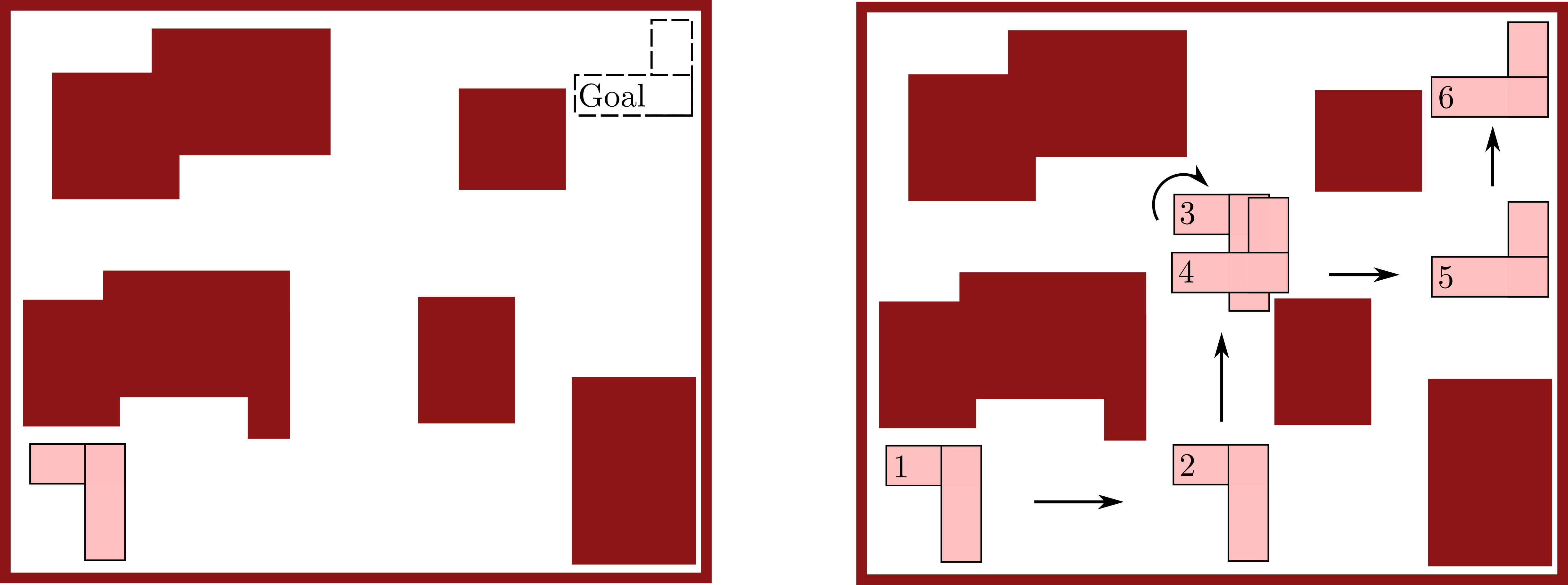
With this setup, the fundamental motion planning problem can be informally stated as follows: given an initial placement of the robot, compute how to gradually move it into a desired goal placement without colliding with any obstacles. As an illustration, consider the workspace in Figure 4.1, where the task is to move an L-shaped robot from its initial position to a target position while avoiding polygonal obstacles. In this case, the output of a motion planning algorithm will be a path through the set of all intermediate transformations of the robot, from start to goal.

Although the motion planning problem is naturally described in the robot’s workspace, it really lives in another space: the set of all rigid-body transformations that describe the robot’s possible placements. As discussed in Chapter 1, this set is referred to as the configuration space or $\mathcal{C}$ -space. In this formulation, obstacles in the workspace induce forbidden regions in $\mathcal{C}$ , and the motion planning problem reduces to finding a continuous path in $\mathcal{C}$ that avoids collisions.

Let us briefly review the notion of configuration space through an example.

Example 4.1.1 (L-shaped Robot).

Consider the L-shaped robot in Figure 4.1. The task is to move it from an initial placement to a goal placement in a two-dimensional world with polygonal obstacles. Suppose the robot is described by a state:

\bm{x}=\begin{bmatrix}x&y&\theta&\dot{x}&\dot{y}&\dot{\theta}\end{bmatrix}^{% \top},

where $(x,y)$ denote position, $\theta$ denotes orientation, and $(\dot{x},\dot{y},\dot{\theta})$ denote velocities. For the simplest version of motion planning, we restrict the attention to the robot’s configuration:

\bm{q}=\begin{bmatrix}x&y&\theta\end{bmatrix}^{\top},

which fully describes its degrees of freedom. In other words, every combination of $(x,y,\theta)$ corresponds to a unique placement of the robot in the workspace, and is called a configuration. This abstraction simplifies the problem: instead of computing a trajectory for the full state, we seek a sequence of collision-free configurations, as shown in the right-side graphic of Figure 4.1. The resulting geometric path in configuration space can then be provided to trajectory optimization methods for refinement—allowing them to incorporate system dynamics—and subsequently to closed-loop control methods (e.g., tracking controllers introduced in Chapter 3) for execution.

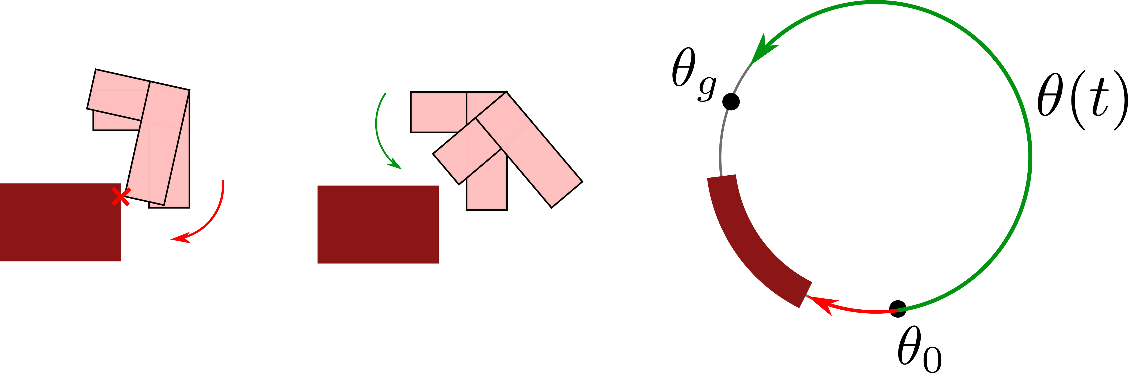
Refer to caption — Figure 4.1: Motion planning in a two-dimensional workspace with obstacles. The task is to move the L-shaped robot from start (bottom-left) to goal (top-right) without collisions.

In this example, the configuration space is $\mathcal{C}=\mathbb{R}^{2}\times\mathcal{S}^{1}\subset\mathbb{R}^{3}$ , where $\mathbb{R}^{2}$ represents the robot’s position in the plane and $\mathcal{S}^{1}$ is the one-dimensional unit circle manifold representing the robot’s orientation. The presence of the manifold $\mathcal{S}^{1}$ reflects the periodicity of the orientation variable $\theta$ , where $\theta$ and $\theta\pm 2\pi k$ are equivalent for all integers $k$ . This periodicity has important practical implications for planning, as the robot can reach the same orientation either by rotating clockwise or counter-clockwise^†^†margin: For instance, a heading change of $\pi/2$ radians can be achieved by turning left by $\pi/2$ or turning right by $3\pi/2$ . . In the scenario depicted in Figure 4.2, suppose the robot has an initial heading $\theta_{0}$ and a goal heading $\theta_{g}$ . If one were to consider only clockwise rotations, there would be no feasible path to the goal without colliding with the obstacle. However, once periodicity is properly accounted for by modeling orientation as $\mathcal{S}^{1}$ , the robot can simply rotate counter-clockwise to reach the goal without collision. Therefore, in this example, the motion planning problem reduces to finding a continuous path in $\mathcal{C}=\mathbb{R}^{2}\times\mathcal{S}^{1}$ that avoids the forbidden regions induced by the obstacles in the workspace.

Crucially, the concept of configuration space generalizes to robots with more complex geometries and higher degrees of freedom (e.g., robotic arms with multiple joints).

Free space in configuration space.

A fundamental concept in motion planning is the free space, denoted by $\mathcal{C}_{\mathrm{free}}$ . Intuitively, $\mathcal{C}_{\mathrm{free}}$ is the set of all robot configurations in which the robot does not collide with any obstacles in the workspace. Formally, let $R(q)\subseteq\mathcal{W}$ denote the set of points in the workspace occupied by the robot when placed at configuration $q$ . The free space is defined as:

\mathcal{C}_{\mathrm{free}}=\{q\in\mathcal{C}\,|\,R(q)\cap\mathcal{O}=% \emptyset\}.

(4.1)

Similarly, the obstacle region in configuration space, denoted by $\mathcal{C}_{\mathrm{obs}}$ , is defined as the complement of the free space:

\mathcal{C}_{\mathrm{obs}}=\{q\in\mathcal{C}\mid R(q)\cap\mathcal{O}\neq% \emptyset\}.

(4.2)

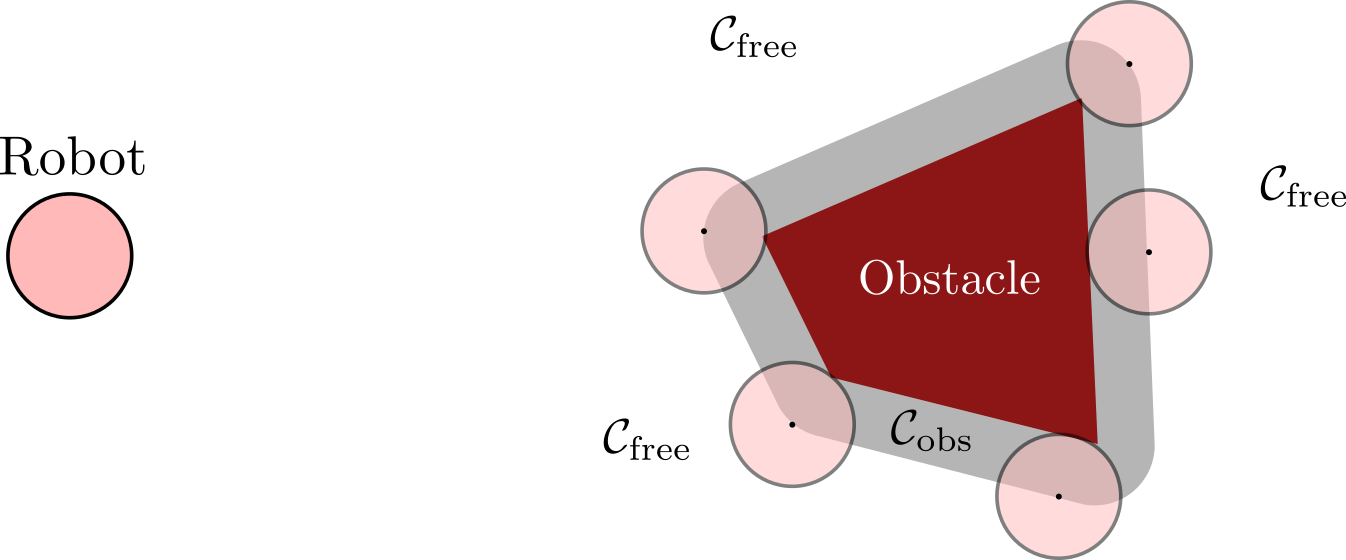
To illustrate these definitions, consider the simple case of a circular robot navigating among polygonal obstacles, as shown in Figure 4.3. Although the robot itself is a disk of nonzero radius, collision checking in configuration space reduces to verifying that a point-like representation of the robot (its configuration) does not intersect the obstacle regions in configuration space. In this case, this equivalence is achieved by inflating the workspace obstacles by the robot’s radius. The red region in the figure represents the obstacle in the physical workspace, $\mathcal{O}$ , whereas the grey region corresponds to the inflated obstacle in configuration space, $\mathcal{C}_{\mathrm{obs}}$ .

Once $\mathcal{C}_{\mathrm{free}}$ (and, correspondingly, $\mathcal{C}_{\mathrm{obs}}$ ) has been computed, the robot’s physical dimensions no longer need to be explicitly considered, and the robot can be treated as a point moving through the configuration space, as illustrated in the previous example. With this abstraction, the geometric complexity of the robot and the environments are absorbed into the structure of the configuration space itself.

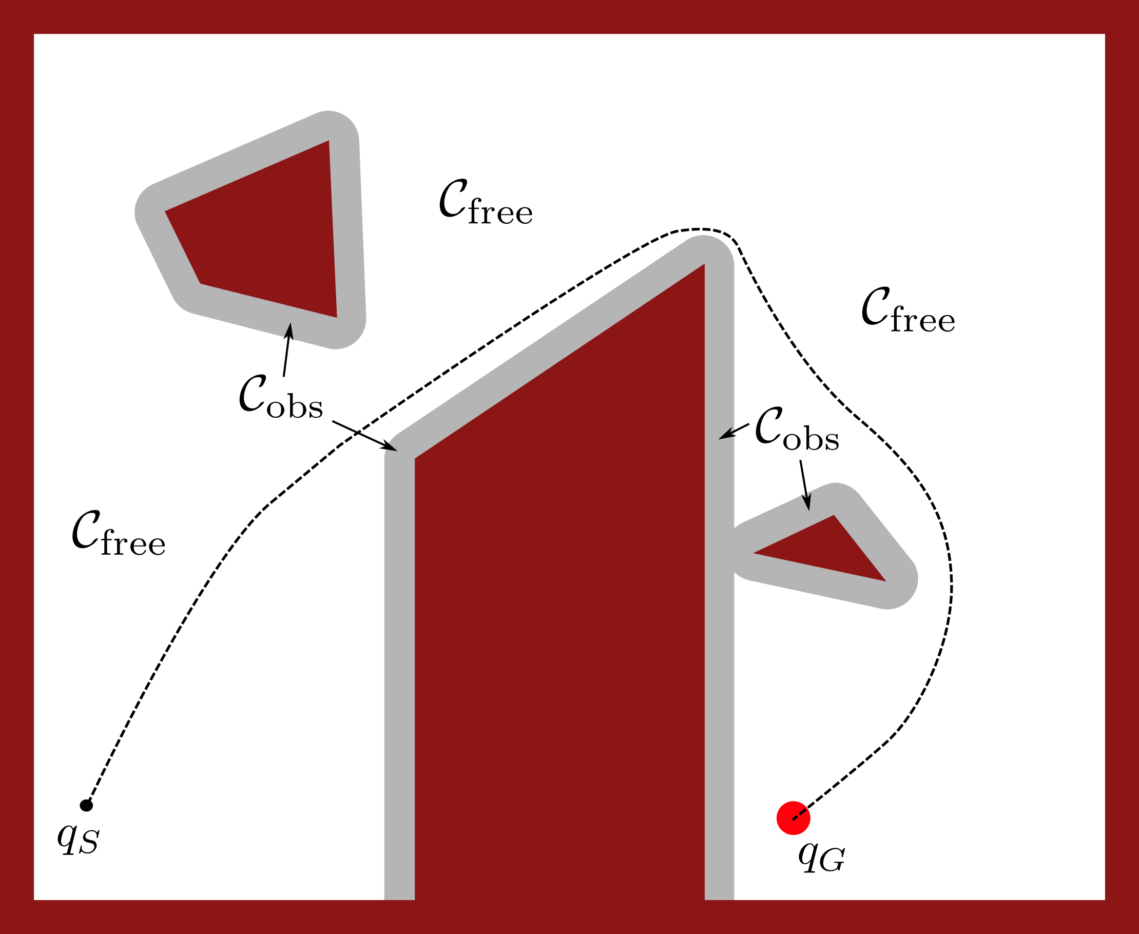
Within this abstracted setting, the motion planning problem reduces to finding a continuous path $\tau:[0,1]\to\mathcal{C}_{\mathrm{free}}$ such that $\tau(0)=q_{\mathrm{S}}$ and $\tau(1)=q_{\mathrm{G}}$ , where $q_{\mathrm{S}}$ and $q_{\mathrm{G}}$ denote the start and goal configurations, respectively. An example is shown in Figure 4.4, where the robot must navigate around forbidden regions in $\mathcal{C}$ -space to reach the goal. By working in configuration space, the problem of collision-free navigation becomes purely geometric, focused on finding a path that avoids the forbidden regions^†^†margin: As we will see in Section 4.4.5, this purely geometric interpretation is true for static environments and without kinodynamic constraints. .

In the remainder of this chapter, we explore various algorithmic strategies that aim to solve either discretized (Section 4.2) or continuous (Sections 4.3-Section 4.5) versions of the motion planning problem.

4.2 Grid-based Motion Planning

A natural way to simplify the motion planning problem is to discretize the robot’s continuous configuration space into a grid. Instead of reasoning about infinitely many possible configurations, we approximate the environment by dividing it into a finite set of cells. Each cell is classified as either free (i.e., collision-free, meaning the robot can occupy it) or forbidden (i.e., meaning it would lead to a collision with an obstacle). The robot is allowed to move between adjacent free cells, and the planning task reduces to finding a sequence of connected free cells that leads from the start to the goal.

This discretization naturally converts motion planning into a graph search problem. Specifically, each free cell in the grid is represented as a vertex in a graph, and an edge is added between two vertices whenever the corresponding cells are adjacent and both free. Formally, we construct a graph $\mathcal{G}=(\mathcal{V},\mathcal{E})$ , where each vertex $v\in\mathcal{V}$ corresponds to a free cell, and each edge $(v,u)\in\mathcal{E}$ corresponds to a valid robot move between adjacent cells. Planning then amounts to finding a path in the graph from the start vertex to the goal vertex.

This perspective is powerful because it allows motion planning to draw on decades of results from graph theory and computer science. Algorithms originally developed for solving shortest-path problems—such as breadth-first search or Dijkstra’s algorithm—can be directly applied to motion planning. In other words, the seemingly geometric problem of “navigating through a space with obstacles” is reduced to the purely combinatorial problem of “finding a path through a graph”. This approach, however, relies on an explicit characterization of $\mathcal{C}_{\mathrm{free}}$ , which is necessary to construct the grid and classify each cell as either free or occupied. In practice, obtaining such an exact characterization is often infeasible—particularly in high-dimensional configuration spaces—thereby motivating alternative strategies, such as sampling-based planning, discussed later in this chapter.

Connectivity and neighborhood structure.

The way adjacency is defined depends on the robot model and the chosen grid structure:

•

In a 4-connected grid, each cell has up to four neighbors (up, down, left, right).
•

In an 8-connected grid, diagonal moves are also allowed, giving each cell up to eight neighbors.
•

More generally, one can consider $k$ -connected neighborhoods (e.g., 16-connected) or hexagonal tilings, trading off simplicity, path quality, and computational cost.

The choice of connectivity has practical consequences. A coarse neighborhood may restrict the robot’s ability to approximate smooth trajectories, while a richer neighborhood increases branching factors and search complexity. Regardless of the specific choice, the key point is that the grid structure induces a well-defined graph on which search algorithms can operate.

4.2.1 Label Correcting Algorithms

Once the motion planning problem has been cast as a graph search, the next step is to design an algorithm that systematically explores the graph to find a path from start to goal. A broad and powerful family of methods for this task is known as label-correcting algorithms.

The term “label” refers to a numerical value associated with each vertex in the graph, which represents the cost of the best-known path from the start vertex to that vertex. At a high level, label correcting algorithms proceed by iteratively refining these cost labels. Initially, only the start vertex has a cost label of zero, while all others are initialized to infinity (or an undefined state). The algorithm proceeds by exploring the graph and updating, or correcting, these labels whenever a better (lower-cost) path to a vertex is discovered.

Formally, let $q_{\mathrm{S}}$ denote the start vertex and $q_{\mathrm{G}}$ the goal vertex^†^†margin: We use the notation $q$ for graph vertices to emphasize the connection between graph search and path planning in configuration space, where $q$ typically denotes a configuration. . For each vertex $q$ , let $C(q)$ represent the label, i.e., the cost of the best path found so far from $q_{\mathrm{S}}$ to $q$ . This value is also known as the cost of arrival.

Label-correcting algorithms operate by maintaining a frontier (also referred to as the alive set or a priority queue) of vertices whose neighbors may still admit cost improvements. At each iteration, a vertex $q$ is extracted from the frontier and expanded. Expansion refers to the process of examining all outgoing edges from $q$ to its neighboring vertices $q^{\prime}$ . For every neighbor^†^†margin: In graph theory, two vertices are denoted as neighbors if they are connected by an edge. $q^{\prime}$ of $q$ , the algorithm attempts to improve (or relax) the current cost estimate associated with $q^{\prime}$ . Specifically, given an edge $(q,q^{\prime})$ with cost $c(q,q^{\prime})$ , the relaxation step verifies whether the path through $q$ offers a lower cost of arrival to $q^{\prime}$ than any previously known path—namely, whether:

C(q)+c(q,q^{\prime})<C(q^{\prime}).

If this condition holds, the label of $q^{\prime}$ (i.e., $C(q^{\prime})$ ) is updated and $q^{\prime}$ is reinserted into the frontier for further exploration. This process continues until no label can be further improved.

General structure of label-correcting algorithms.

All algorithms in this family share the following structure:

•

Initialization: Set $C(q_{\mathrm{S}})=0$ and $C(q)=\infty$ for all other vertices $q$ . Initialize the frontier with the start vertex $Q=\{q_{\mathrm{S}}\}$ .
•
Main Loop: Until the frontier $Q$ is not empty, repeat:
1. 1.
  
  Extract a vertex $q$ from the frontier $Q$ according to a specific selection rule^†^†margin: The choice of selection rule is the main distinguishing factor between different label-correcting algorithms. .
2. 2.
  For each neighbor $q^{\prime}$ of $q$ , perform the relaxation step, i.e.:
  1. (a)
    
    Check if $C(q)+c(q,q^{\prime})<C(q^{\prime})$ .
  2. (b)
    
    If so, update $C(q^{\prime})\leftarrow C(q)+c(q,q^{\prime})$ and add $q^{\prime}$ to the frontier $Q$ if it is not already present.
•

Termination: The algorithm terminates when the frontier is empty. At this point, $C(q)$ contains the cost of the shortest path from $q_{\mathrm{S}}$ to each reachable vertex $q$ .

The pseudocode for the general structure of a label-correcting algorithm is provided in Algorithm 1.

Data:

q_{\mathrm{S}}

q_{\mathrm{G}}

, directed graph

\mathcal{G}=(\mathcal{V},\mathcal{E})

, edge costs

c(\cdot,\cdot)

, selection rule

\mathsf{Select}

Result: Shortest path from

q_{\mathrm{S}}

q_{\mathrm{G}}

(if reachable)

for $q\in\mathcal{V}\setminus\{q_{\mathrm{S}}\}$ do

C(q)\leftarrow\infty

C(q_{\mathrm{S}})\leftarrow 0

Q\leftarrow\{q_{\mathrm{S}}\}

/* Initialize priority queue */

while $Q$ is not empty do

q\leftarrow\mathsf{Select}(Q)

;

Q.\mathrm{remove}(q)

for $q^{\prime}\in\{\,u\mid(q,u)\in\mathcal{E}\,\}$ do

\tilde{C}\leftarrow C(q)+c(q,q^{\prime})

if $\tilde{C}<C(q^{\prime})$ then

C(q^{\prime})\leftarrow\tilde{C}

;

\mathrm{parent}(q^{\prime})\leftarrow q

if $q^{\prime}\neq q_{\mathrm{G}}$ and $q^{\prime}\notin Q$ then

Q.\mathrm{add}(q^{\prime})

if $C(q_{\mathrm{G}})=\infty$ then

return N.A.

/* Goal unreachable */

else

/* Reconstruct path by backtracking parents */

\mathrm{path}\leftarrow[\,]

;

q\leftarrow q_{\mathrm{G}}

while $q\neq q_{\mathrm{S}}$ do

\mathrm{path}

\mathrm{prepend}(q)

;

q\leftarrow\mathrm{parent}(q)

return $\mathrm{path}$

Algorithm 1 Structure of a Label-Correcting Algorithm

The role of the selection rule.

The selection rule for choosing the next vertex to expand is one of the key factors that differentiates various label-correcting algorithms, ultimately defining their efficiency and performance. Several classical search methods can be seen as special cases of the label-correcting framework, for example:

•

Depth-First Search (DFS): in DFS ( Figure 4.5), the frontier is managed as a stack (last-in, first-out). This means that the algorithm always continues along the most recently discovered path before backtracking. DFS is appealing for its simplicity and low memory footprint, since the number of active nodes is proportional to the depth of the search. However, DFS is exposed to the risk of getting trapped in deep but unproductive branches of the search tree, leading to poor performance in finding the shortest path.

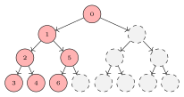
Figure 4.5: Depth-first search
•

Breadth-First Search (BFS): in BFS ( Figure 4.6), the frontier is a queue (first-in, first-out). The algorithm expands all nodes at a given “depth” before moving on to the next, effectively exploring the graph in concentric layers around the start node. Compared to DFS, BFS requires significantly more memory, as it must store all frontier nodes at a given depth.

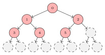
Figure 4.6: Breadth-first search
•

Dijkstra’s Algorithm (also known as Best-First Search): in Dijkstra’s algorithm (Algorithm 4.1), the frontier is a priority queue ordered by the tentative label $C(q)$ , i.e., the best cost of arrival discovered so far. At each iteration, the vertex with the smallest label is selected for expansion. Formally, we express this greedy selection of the next vertex as:

$\mathsf{Select}(Q)=\arg\min_{q\in Q}C(q).$ (4.3)

A key property of Dijkstra’s algorithm is that once a vertex is extracted from the priority queue, its label is guaranteed to be final and optimal. In other words, each node will be expanded at most once, leading to a more efficient exploration of the graph. Because of this, Dijkstra’s algorithm provides the foundation for many widely used planning methods such as $A^{*}$ and $D^{*}$ .

⬇

def dijkstra(start_node, edges):

visited = set()

Q = [(0, start_node)]

while Q:

current_cost, current_node = heapq.heappop(Q)

if current_node in visited:

continue

visited.add(current_node)

for neighbor, edge_cost in edges[current_node]:

if neighbor in visited:

continue

new_cost = current_cost + edge_cost

if new_cost < neighbor.cost:

neighbor.cost = new_cost

neighbor.parent = current_node.idx

heapq.heappush(Q, (new_cost, neighbor))

Algorithm 4.1: Python implementation of Dijkstra’s algorithm. See this code used in the context of motion planning in the repository github.com/StanfordASL/pora-exercises in the notebook ch04/prm_star.ipynb.

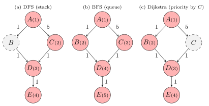
To make the differences between these search strategies more concrete, consider the simple graph in Figure 4.7. In this example, the start vertex is $A$ and the goal vertex is $E$ . The numbers in parentheses indicate the order of expansion for each of the three search strategies, and the numbers next to each edge indicate the cost of traversing that edge. By observing the order of expansion, we can see how each strategy explores the graph differently, with DFS going deep into one branch, BFS exploring all nodes at the current depth before moving deeper, and Dijkstra’s algorithm expanding nodes based on the lowest cumulative cost.

diagram — Figure 4.7: Effect of the selection rule on exploration order. Numbers inside nodes indicate the order of expansion (removal from the frontier). DFS follows the most recently discovered branch and may yield a suboptimal-cost route; BFS explores all nodes at the current depth before proceeding deeper; Dijkstra expands in order of lowest cost from the start node.

Beyond Dijkstra: toward more informed search for motion planning.

Dijkstra’s algorithm is one of the most widely used methods for graph search, owing to its simplicity and the guarantee that it always finds an optimal path, if one exists²⁴24. Bertsekas, D. Dynamic Programming and Optimal Control. Athena Scientific, 2000.. In particular, Dijkstra is a correct algorithm, in that it always finds a least-cost path from the start node to the goal node, provided such a path exists.

Theorem 4.1 (Correctness of a graph search algorithm; Bertsekas (2000)²2. Bertsekas, D. Dynamic Programming and Optimal Control. Athena Scientific, 2000.).

If a feasible path exists from $q_{\mathrm{S}}$ to $q_{\mathrm{G}}$ , then the algorithm terminates in finite time with $C(q_{\mathrm{G}})$ equal to the optimal cost of traversal, $C^{*}(q_{\mathrm{G}})$ .

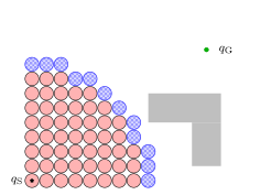
While this property makes Dijkstra appealing, its exploration strategy may result in significant wasted effort. By always expanding the frontier node with the smallest accumulated cost of arrival, Dijkstra effectively explores the search space in “cost contours” radiating outward from the start. This strategy guarantees optimality for the path that is returned, but may expand many vertices that are irrelevant for reaching the goal, a drawback that becomes especially pronounced in the large and structured graphs typical of motion planning (see Figure 4.8).

These limitations motivated the development of more informed search strategies that incorporate additional guidance toward the goal. The most influential among these are the A* algorithm, which augments Dijkstra with heuristic estimates of the remaining cost to the goal, and its dynamic extension, the D* algorithm, which adapts the search as new information about the environment becomes available.

The A* algorithm.

The $A^{*}$ algorithm improves upon Dijkstra’s selection rule by augmenting the cost of arrival with a heuristic estimate of the cost-to-go, i.e., the cost from the current node to the goal. Formally, instead of expanding the vertex that minimizes $C(q)$ , $A^{*}$ expands the vertex that minimizes:

f(q)=C(q)+h(q),

(4.4)

where $h(q)$ is a heuristic function estimating the optimal remaining cost from $q$ to the goal. Consequently, the relaxation step for each neighbor $q^{\prime}$ of $q$ is also strengthened to update $f(q^{\prime})$ rather than just the cost of arrival $C(q^{\prime})$ :

f(q^{\prime})\leftarrow\min\big{(}f(q^{\prime}),C(q)+c(q,q^{\prime})+h(q^{% \prime})\big{)}.

(4.5)

As long as $h(\cdot)$ is admissible (i.e., it never overestimates the true cost-to-go), $A^{*}$ is guaranteed to return an optimal path. Intuitively, underestimating the cost-to-go ensures that nodes are not prematurely discarded, which could otherwise lead to suboptimal solutions. In practice, heuristics such as the Euclidean or Manhattan distance to the goal often reduce the number of vertices explored, since the search is biased toward the target rather than expanding uniformly in all directions. This makes $A^{*}$ one of the most widely used graph search algorithms for the purposes of motion planning.

The D* algorithm.

In many robotic applications, the environment is only partially known in advance, and new information (such as previously unseen obstacles) may be discovered during execution. Recomputing an $A^{*}$ search from scratch each time the map changes can be computationally challenging. The $D^{*}$ algorithm (Dynamic A*) addresses this challenge by incrementally repairing the solution when changes are detected. Rather than discarding the existing search tree, $D^{*}$ efficiently updates cost labels and frontier priorities, reusing past computations whenever possible. This makes it particularly suitable for autonomous navigation in dynamic or uncertain environments, where the robot must adapt its plan online as new information is gathered. For an in-depth treatment of $D^{*}$ , we refer the reader to Stentz (1995)³3. Stentz, A. “The focussed D* algorithm for real-time replanning.” In 14th International Joint Conference on Artificial Intelligence, 1652–1659, 1995..

Pros and cons of grid-based planning.

Grid-based planning methods offer several appealing advantages that explain their long-standing popularity in robotics. Perhaps the most important benefit is their simplicity: the underlying idea of discretizing the configuration space into cells and treating planning as a graph search problem is straightforward to implement and reason about. Once the grid is constructed, classical search algorithms such as DFS, BFS, or Dijkstra can be directly applied. This also makes grid-based methods relatively fast in certain settings, particularly when the resolution of the grid is well-matched to the scale of the environment and the complexity of the obstacles.

Despite these advantages, grid-based methods come with important limitations. A first challenge is that they are inherently resolution dependent. If the grid resolution is too coarse, narrow passages or fine obstacle boundaries may be missed, and the planner may fail to find a feasible solution even if one exists in the continuous space. On the other hand, using a very fine grid increases the computational burden significantly, as the number of grid cells grows rapidly with finer resolution. Thus, achieving the right tradeoff between resolution and tractability is nontrivial.

A second drawback is that grid-based planning scales poorly with robot complexity. While it is effective for simple 2D robots moving in two-dimensional workspaces (i.e., where configuration space and workspace coincide), the size of the grid grows exponentially with the number of degrees of freedom (DOFs) of the robot. Moreover, grid-based planning requires an exact characterization of the free space $\mathcal{C}_{\mathrm{free}}$ , which is often difficult to compute in high-dimensional configuration spaces. These limitations motivate the development of sampling-based methods, which are discussed in Section 4.4. As a result, grid-based methods are primarily used for robots with few DOFs or for simplified planning problems where the dimensionality of the configuration space is deliberately reduced.

In summary, grid-based planning remains a widely used and important approach, particularly for low-dimensional problems. However, its reliance on discretization and its exponential scaling with dimension limit its applicability to more complex robotic systems.

4.3 Combinatorial Motion Planning

In this section, we return to the continuous formulation of the motion planning problem and explore combinatorial approaches. The key idea is to construct an exact representation of the connectivity of the free space $\mathcal{C}_{\mathrm{free}}$ without resorting to approximations. Instead of discretizing the space arbitrarily, combinatorial methods compute a roadmap that captures the essential topological structure of $\mathcal{C}_{\mathrm{free}}$ to enable planning in continuous spaces.

Due to this property, combinatorial motion planning algorithms are referred to as exact, as they find paths through the continuous configuration space without resorting to approximations. Combinatorial planners are also complete, meaning they are guaranteed to find the optimal path if one exists, or correctly report failure otherwise. This is in contrast to grid-based planners, which are only resolution complete, guaranteeing a solution only if one exists at the chosen discretization resolution.

However, like grid-based methods, combinatorial planning becomes computationally challenging in high-dimensional configuration spaces, since computing the exact geometry of $\mathcal{C}_{\mathrm{free}}$ , and its decomposition into a roadmap, is often prohibitively expensive. As a result, such approaches are best suited for robots with a small number of degrees of freedom or for low-dimensional planning problems.

The roadmap.

A roadmap is a graph $\mathcal{G}=(\mathcal{V},\mathcal{E})$ embedded in the configuration space, where each vertex $q\in\mathcal{V}$ corresponds to a configuration in $\mathcal{C}_{\mathrm{free}}$ , and each edge $(q,q^{\prime})\in\mathcal{E}$ represents a continuous, collision-free path between the corresponding configurations. Let $\mathcal{S}\subset\mathcal{C}_{\mathrm{free}}$ denote the set of all configurations represented by the vertices in $\mathcal{G}$ . For $\mathcal{G}$ to be a valid roadmap, it must satisfy two key conditions that ensure it accurately represents the structure of $\mathcal{C}_{\mathrm{free}}$ :

1.

Accessibility: from any configuration $q\in\mathcal{C}_{\mathrm{free}}$ , it must be simple to compute a continuous, collision-free path to any configuration $s\in\mathcal{S}$ . Typically, $s$ is chosen as the nearest vertex to $q$ (assuming $\mathcal{C}$ is a metric space). This condition ensures that every configuration in the free space can be connected to the roadmap without leaving $\mathcal{C}_{\mathrm{free}}$ .
2.

Connectivity-preserving: using the accessibility condition, it must be possible to connect any two configurations $q_{\mathrm{S}},q_{\mathrm{G}}\in\mathcal{C}_{\mathrm{free}}$ to some $s_{1},s_{2}$ in the roadmap, respectively. The connectivity-preserving property requires that if there exists a continuous, collision-free path between $q_{\mathrm{S}}$ and $q_{\mathrm{G}}$ in $\mathcal{C}_{\mathrm{free}}$ , then there must also exist a corresponding path between $s_{1}$ and $s_{2}$ in the roadmap $\mathcal{G}$ . In other words, no feasible path in $\mathcal{C}_{\mathrm{free}}$ is lost because the roadmap fails to capture the underlying connectivity of the free space. This property is essential for the completeness of combinatorial planning algorithms.

Once these conditions are satisfied, the roadmap provides an exact representation of the planning problem, where vertices correspond to representative configurations in accessible regions of $\mathcal{C}_{\mathrm{free}}$ , and edges encode the connectivity between them. Motion planning then reduces to a graph search problem, where the start and goal configurations are connected to the roadmap and a path is searched for in the resulting graph.

While this structure may appear similar to the grid-based approach discussed earlier, the key distinction lies in how the space is represented. A roadmap is constructed to capture the true geometry and connectivity of $\mathcal{C}_{\mathrm{free}}$ , rather than imposing a fixed discretization of $\mathcal{C}$ onto a uniform grid. In other words, vertices in a roadmap can correspond to any configuration within the free space, allowing feasible paths to always be preserved in the graph representation, whereas grid-based methods may fail to represent certain valid paths due to the coarseness of the underlying discretization. This two-step procedure—roadmap construction followed by graph search—provides a powerful and general framework for motion planning^†^†margin: For an in-depth treatment of the concepts of roadmaps, and a formal definition of the requirements for completeness and optimality, see LaValle (2006)⁴4. LaValle, S. M. Planning Algorithms. Cambridge University Press, 2006.. .

4.3.1 Cell Decomposition

As discussed above, combinatorial methods must construct a finite data structure that exactly encodes the planning problem. One way to achieve this is through cell decomposition methods, which partition the free space $\mathcal{C}_{\mathrm{free}}$ into a finite collection of regions, called cells, that can be used to construct a roadmap.

A useful way to think about cell decompositions is through three key properties that make them suitable for motion planning:

1.

Trivial connectivity within cells: computing a path from one configuration to another inside a cell must be easy. For instance, if every cell is convex, then any two points in the cell can be connected by a straight-line segment that remains in $\mathcal{C}_{\mathrm{free}}$ .
2.

Adjacency extraction: it must be straightforward to determine which cells are adjacent to one another, so that a roadmap can be built by connecting neighboring cells.
3.

Efficient query location: for a given initial and goal configuration $(q_{\mathrm{S}},q_{\mathrm{G}})$ , it should be efficient to determine which cells contain them.

When these conditions are satisfied, the motion planning problem reduces to a graph search problem, where vertices correspond to representative configurations in each cell, and edges connect neighboring cells.

Vertical cell decomposition.

A widely used technique for 2D environments is the vertical decomposition, also called trapezoidal decomposition. Suppose the obstacles are polygonal, and let $P$ denote the set of vertices defining $\mathcal{C}_{\mathrm{obs}}$ . At each vertex $p\in P$ , rays are extended vertically upward and downward through $\mathcal{C}_{\mathrm{free}}$ until they intersect either another obstacle or the workspace boundary. Depending on the local geometry, four distinct cases arise, corresponding to whether a vertical extension is possible upward, downward, in both directions, or in neither, as illustrated in Figure 4.9.

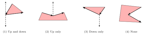
The result of this process, illustrated in Figure 4.10, is a decomposition of $\mathcal{C}_{\mathrm{free}}$ into a collection of 2-cells (open trapezoids and degenerate triangles) and 1-cells (open vertical line segments forming the boundaries between trapezoids).

Once the decomposition is available, a roadmap $\mathcal{G}=(\mathcal{V},\mathcal{E})$ can be constructed. For each 2-cell $C_{i}$ , a representative sample point $q_{i}\in C_{i}$ is chosen—commonly the centroid, though the exact choice is not critical. Each 1-cell is also assigned a sample point. These points are visualized as black dots in Figure 4.10. The roadmap graph is then defined as follows: every cell corresponds to a vertex, and for each 2-cell, edges are added to connect its sample point with the sample points of adjacent 1-cells lying on its boundary.

By construction, both the accessibility and the connectivity conditions are satisfied, i.e., every sample point is accessible via a straight-line path within its cell, and any two adjacent cells are connected by an edge in the roadmap. Thus, the roadmap provides an exact representation of the planning problem. Once the roadmap is constructed, the explicit cell decomposition is no longer needed, and planning reduces to connecting $q_{\mathrm{S}}$ and $q_{\mathrm{G}}$ to the roadmap and performing a graph search.

Example 4.3.1 (2D Cell Decomposition).

Consider the two-dimensional configuration space in Figure 4.10. Using vertical decomposition, the free space is partitioned into trapezoids and triangles separated by vertical segments. A roadmap is obtained by placing representative vertices (shown as black dots) inside the cells and along their shared boundaries, and connecting them according to adjacency. To solve a motion planning query, start and goal configurations are connected to their respective cells, and a path is found via a standard graph search algorithm.

4.3.2 Other Roadmap Construction Methods

Beyond cell decomposition, several other methods have been developed to construct roadmaps, often exploiting geometric properties of the free space.

For instance, maximum clearance roadmaps attempt to maintain as much distance as possible from obstacles, effectively following the “skeleton” of the free space. A well-known example is the generalized Voronoi diagram, where the roadmap consists of points in $\mathcal{C}_{\mathrm{free}}$ equidistant to at least two obstacles. Such roadmaps have the advantage of producing paths that maximize safety margins, which is particularly useful for robots operating in tight or uncertain environments. Another approach is the shortest path roadmap, which constructs the roadmap by connecting pairs of points in $\mathcal{C}_{\mathrm{free}}$ with the shortest possible paths that avoid obstacles. For an in-depth discussion of these and other roadmap construction techniques, we refer the reader to LaValle (2006)⁵5. LaValle, S. M. Planning Algorithms. Cambridge University Press, 2006.. Each of these roadmap constructions provides a different balance between ease of computation, path quality, and robustness. The choice of method depends on the geometry of the robot and environment, as well as the requirements of the task at hand.

4.4 Sampling-based Motion Planning

The limitations of combinatorial and grid-based methods, particularly their computational complexity in high-dimensional spaces, have motivated the development of sampling-based motion planning algorithms. At a high level, these algorithms explicitly avoid the need for an explicit representation of $\mathcal{C}_{\mathrm{free}}$ and $\mathcal{C}_{\mathrm{obs}}$ , instead relying on random sampling to capture the structure of the configuration space. To do so, sampling-based methods combine random sampling in $\mathcal{C}$ -space with black-box collision detection algorithms that can determine whether a configuration or path segment is collision-free (i.e., lies in $\mathcal{C}_{\mathrm{free}}$ ). By incrementally connecting such collision–free samples, sampling-based methods are able to build a roadmap or tree structure that captures the feasible connectivity of the free space without ever explicitly representing it, in practice ensuring significant computational speed ups. This paradigm offers several advantages:

•

Conceptual simplicity: algorithms are relatively easy to understand and implement.
•

Generality: the same framework applies to different robots and environments.
•

Extensibility: the methodology can be extended beyond purely geometric settings to handle kinodynamic planning, differential constraints, and uncertainty.

At the same time, sampling–based methods have inherent limitations. Unlike exact combinatorial approaches, they generally offer weaker guarantees regarding the existence or quality of the resulting solution. Moreover, it may be challenging to know a priori how many samples are needed to find a solution, or to ensure that the planner will find a solution if one exists. On the theoretical side, most methods offer probabilistic guarantees rather than deterministic ones: they are probabilistically complete (i.e., if a feasible path exists, the probability of finding one approaches 1 as the number of samples $n$ tends to infinity) and, for certain variants, asymptotically optimal (i.e., if $C_{n}$ is the cost of the best path found after $n$ samples and $C^{\star}$ is the optimal cost, then $C_{n}$ tends to $C^{\star}$ with probability 1). Both properties are asymptotic and probabilistic in nature, as they provide no finite-sample guarantee but only that the probability of failure (or of suboptimality) vanishes as $n$ grows. These properties will be discussed in more detail in Section 4.4.3.

Traditionally, sampling-based motion planning algorithms fall into two main approaches: probabilistic roadmaps (PRMs) and rapidly-exploring random trees (RRTs). PRMs are multi-query planners, as their precomputed structures can be reused to answer multiple planning problems in the same environment. By contrast, RRTs are single-query planners, designed to find a solution for a specific start–goal pair $(q_{\mathrm{S}},q_{\mathrm{G}})$ in a given free configuration space $\mathcal{C}_{\mathrm{free}}$ . Despite this distinction, both families of algorithms share two fundamental components. The first is a collision detection routine, $\texttt{CollisionFree}(q)$ , which determines whether a configuration $q$ lies within the free space $\mathcal{C}_{\mathrm{free}}$ . The second is a local planner, $\texttt{LocalPlanner}(q,q^{\prime})$ , which produces a short path segment—often a straight line in configuration space or a dynamically feasible motion—and verifies its validity by checking for collisions.

Below, we provide an overview of PRMs and RRTs, along with their theoretical properties and practical considerations.

4.4.1 Probabilistic Roadmaps (PRMs)

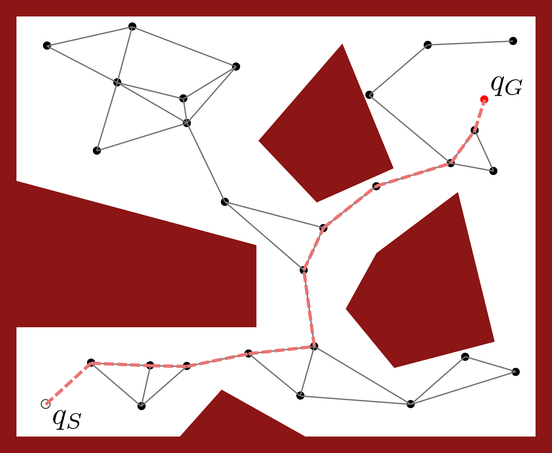
PRMs are among the most influential sampling–based methods for motion planning. At a high level, PRMs are a multi-query planner that constructs a roadmap in the configuration space by randomly sampling configurations and connecting them to form a graph. The PRM algorithm consists of two main phases: a construction phase and a query phase. During the construction phase, the algorithm samples a set of configurations $\{q_{1},q_{2},\ldots,q_{n}\}$ from $\mathcal{C}_{\mathrm{free}}$ using a uniform or biased sampling strategy. Each sampled configuration is then used to construct a roadmap that encodes the connectivity of the free space. As a result, once constructed, the roadmap can be queried to solve multiple planning problems in the same environment by simply attaching start and goal configurations to the roadmap and running a graph search.

Formally, the PRM algorithm can be summarized as follows:

1.
Construction Phase:
1. (a)
  
  Sample $n$ configurations $\{q_{1},q_{2},\ldots,q_{n}\}$ from $\mathcal{C}$ and discard those that lie in $\mathcal{C}_{\mathrm{obs}}$ using the collision detection method $\texttt{CollisionFree}(q)$ .
2. (b)
  
  Draw an edge between each pair of configurations $q_{i}$ and $q_{j}$ according to a chosen connection rule—for example, if they are within a certain distance threshold $r$ , i.e., $||q_{i}-q_{j}||\leq r$ , and if the local planner $\texttt{LocalPlanner}(q_{i},q_{j})$ finds a collision-free path between them, e.g., a straight line segment in $\mathcal{C}$ -space.
2.

Query Phase: given a query $(q_{\mathrm{S}},q_{\mathrm{G}})\in\mathcal{C}_{\mathrm{free}}$ , connect $q_{\mathrm{S}}$ and $q_{\mathrm{G}}$ to the nearest nodes in the roadmap using the local planner, and then use a graph search algorithm (e.g., Dijkstra’s or $A^{*}$ ) to find a path from $q_{\mathrm{S}}$ to $q_{\mathrm{G}}$ through the roadmap.

Figure 4.11 illustrates an example of the PRM algorithm in a simple 2D environment.

Design considerations.

The effectiveness of PRM depends on several key design decisions that shape both its computational performance and its ability to capture the connectivity of the free space. A first consideration concerns the sampling strategy. The most straightforward approach is to generate configurations uniformly at random in the configuration space and retain only those that lie in $\mathcal{C}_{\mathrm{free}}$ . While this method provides unbiased coverage, it may perform poorly in environments dominated by narrow passages, since these regions occupy little volume and are therefore rarely sampled. To address this limitation, various biased sampling strategies have been proposed, which aim to increase the likelihood of sampling configurations in challenging areas of the configuration space. More generally, heuristic biasing strategies can direct samples toward regions that are likely to be relevant for specific planning tasks, trading uniformity for effectiveness in complex environments.

Another important design choice is the method used to connect sampled configurations. Two rules are most common: the fixed-radius rule, where each vertex attempts to connect to all samples within a ball of radius $r$ , and the $k$ -nearest neighbor rule, where each vertex connects to its $k$ closest samples. As will be discussed in the remainder of this chapter, both connection rules are supported by theoretical results that tie the values of $r$ and $k$ to the number of samples and the dimensionality of the space (see, e.g., Karaman and Frazzoli (2011)⁶6. Karaman, S., Frazzoli, E. “Sampling-based Algorithms for Optimal Motion Planning.” Int. Journal of Robotics Research 30(7), 846–894, 2011.). These results ensure that, as the number of samples grows, the roadmap becomes sufficiently connected to capture the topology of $\mathcal{C}_{\mathrm{free}}$ without introducing an excessive number of samples

Characteristics of PRMs.

The probabilistic roadmap framework is particularly well suited to environments that remain static across multiple planning queries. Since the construction of the roadmap can be computationally demanding—dominated by nearest-neighbor queries and collision checking—it is most effective when the investment in preprocessing can be amortized over many queries posed in the same workspace. In these contexts, the roadmap serves as a reusable data structure that compactly encodes the connectivity of the free space, enabling queries to be answered quickly with standard graph search algorithms.

For these reasons, PRM has become a method of choice in domains where multiple planning queries must be solved in high-dimensional but largely static environments. Its strength lies not in producing a single solution quickly, but in building a reusable structure that captures the topology of the free space and can then be reused to efficiently solve many queries.

Overall, PRM-like motion planning algorithms are widely recognized to find “good” paths in practice, even in high-dimensional configuration spaces. However, this may require a large number of expensive collision checks, thus incurring significant computational costs.

4.4.2 Rapidly-Exploring Random Trees (RRTs)

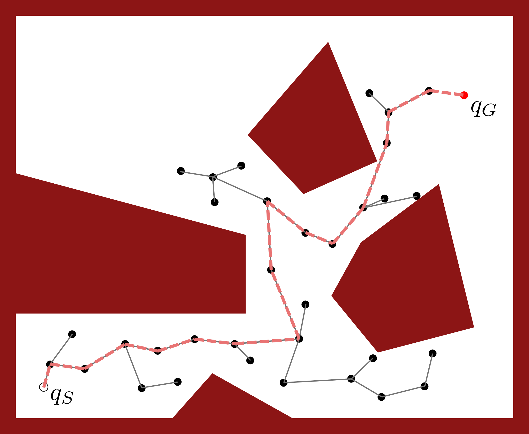
RRT is a foundational sampling–based algorithm designed for single-query motion planning. In contrast to the precomputation strategy of PRMs, RRT incrementally grows a tree^†^†margin: A tree is a special type of graph that is connected and acyclic. In other words, there is exactly one path between any two vertices in a tree. —denoted $\mathcal{T}=(\mathcal{V},\mathcal{E})$ —rooted at the initial configuration $q_{\mathrm{S}}$ , seeking to connect it to a specified goal configuration $q_{\mathrm{G}}$ . As a result, RRT is particularly well suited for scenarios in which only a single query needs to be solved, such as when the environment dynamically changes.

RRT proceeds iteratively, where each iteration consists of the following steps:

1.

Sample a random configuration $q_{\mathrm{rand}}$ from the configuration space $\mathcal{C}$ .
2.

Find the nearest vertex $q_{\mathrm{near}}$ in the tree $\mathcal{T}$ to the sampled configuration $q_{\mathrm{rand}}$ under an appropriate distance metric $d(\cdot,\cdot)$ (e.g., Euclidean distance).
3.

Generate a new configuration $q_{\mathrm{new}}$ by moving from $q_{\mathrm{near}}$ toward $q_{\mathrm{rand}}$ , ensuring that the motion from $q_{\mathrm{near}}$ to $q_{\mathrm{new}}$ is collision-free.
4.

Update the tree $\mathcal{T}$ by adding $q_{\mathrm{new}}$ as a new vertex and connecting it to $q_{\mathrm{near}}$ with an edge $(q_{\mathrm{near}},q_{\mathrm{new}})$ .

The algorithm continues expanding the tree until a vertex is added that is sufficiently close to the goal configuration $q_{\mathrm{G}}$ ^†^†margin: This proximity can be verified, for example, by attempting to connect the newly added vertex to the goal and checking whether the connection is collision-free. If successful, the algorithm terminates. . At that point, a path from $q_{\mathrm{S}}$ to $q_{\mathrm{G}}$ can be extracted by backtracking through the tree. If after a budget of $N$ iterations no feasible connection to the goal is found, the algorithm terminates with failure.

Figure 4.12 illustrates an example of the RRT algorithm in a simple 2D environment.

Voronoi bias.

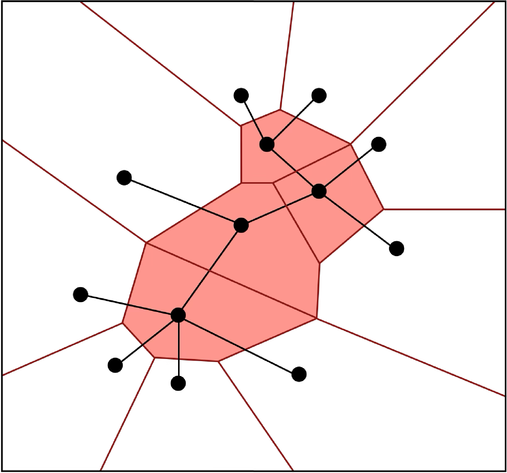
A key insight into RRT’s efficiency comes from interpreting its sampling dynamics through the lens of Voronoi diagrams (Figure 4.13). Each vertex in the tree $\mathcal{T}$ defines a Voronoi cell in configuration space, consisting of all points closer to that vertex than to any other. Since random samples are uniformly distributed, the probability of expanding a given vertex is proportional to the volume of its Voronoi cell. Vertices on the frontier of the tree tend to own large cells, and therefore are more likely to be selected for expansion. This Voronoi bias implicitly drives the tree outward, rapidly exploring uncovered regions without requiring any explicit mechanism for frontier selection.

Overall, RRT provides a powerful framework for single-query motion planning. Specifically, RRT-like motion planning algorithms are widely used in practice due to their ability to find feasible paths quickly in high-dimensional spaces. However, the paths produced by RRT are often suboptimal. Its extensions, particularly RRT^∗ and its variants, combine RRT’s exploratory power with provable guarantees on optimality, making them widely used in practical applications. Importantly, RRT (as well as PRM) does not require an explicit characterization of $\mathcal{C}_{\mathrm{free}}$ , which is key to its scalability to higher-dimensional $\mathcal{C}$ spaces.

4.4.3 Theoretical Guarantees

Both PRM and RRT algorithms come with theoretical guarantees that underpin their effectiveness in motion planning tasks. Specifically, we consider two key properties which formalize the sense in which planners like PRM, RRT, and their related extensions PRM^∗ and RRT^∗ succeed in the limit of large sampling budgets: probabilistic completeness and asymptotic optimality.

Probabilistic completeness.

A planner is said to be probabilistically complete if, whenever a feasible path exists, the probability that the algorithm fails to find one approaches zero as the number of samples $n$ tends to infinity. Both PRM and RRT satisfy probabilistic completeness under reasonable assumptions on the configuration space and the sampling process^†^†margin: Intuitively, the sampling distribution must assign nonzero probability to every open subset of the free space. .

While an in-depth treatment of probabilistic completeness is beyond the scope of this chapter, we refer the reader to Kavraki et al. (1996)⁷7. Kavraki, L. E., Svestka, P., J.-C. Latombe, Overmars, M. H. “Probabilistic roadmaps for path planning in high-dimensional configuration spaces.” IEEE Transactions on Robotics and Automation 12(4), 566–580, 1996. and LaValle (1998)⁸8. LaValle, S. M. Rapidly-Exploring Random Trees: A New Tool for Path Planning. 1998., which establish these guarantees for PRM, RRT, and related algorithms.

Asymptotic optimality.

A planner is asymptotically optimal if, as the number of samples $n$ tends to infinity, the probability that cost of the best path found by the algorithm converges to the optimal cost approaches one. Achieving asymptotic optimality requires careful control of the connectivity of the underlying random graph. If connections are too sparse, the graph may fail to capture near-optimal paths. If connections are too dense, computational costs may increase significantly. Thus, guarantees of asymptotic optimality rely on choosing a connection radius that decreases at an appropriate rate relative to the number of samples to balance these competing effects.

Karaman and Frazzoli (2011)⁹9. Karaman, S., Frazzoli, E. “Sampling-based Algorithms for Optimal Motion Planning.” Int. Journal of Robotics Research 30(7), 846–894, 2011. provided the first rigorous study of asymptotic optimality for sampling-based planners. In particular, they proved the following result for PRM^∗:

Theorem 4.1.

If the connection radius $r(n)$ satisfies:

r(n)\geq\gamma\left(\frac{\log n}{n}\right)^{1/d},

where $d$ is the dimension of the configuration space and $\gamma$ is a constant that depends only on $d$ and $\mathcal{C}_{\mathrm{free}}$ , then the cost of the best path returned by $PRM^{*}$ after $n$ samples converges to the optimal cost with probability one as $n\to\infty$ .

Karaman and Frazzoli (2011)¹⁰10. Karaman, S., Frazzoli, E. “Sampling-based Algorithms for Optimal Motion Planning.” Int. Journal of Robotics Research 30(7), 846–894, 2011. also introduced an asymptotically optimal variant of RRT, called RRT^∗, which incorporates a rewiring step to improve path quality over time.

Example 4.4.1 (PRM* in 2D Workspace).

Explore ch04/prm_star.ipynb in the repository github.com/StanfordASL/pora-exercises for an example implementation of the PRM* algorithm that is asymptotically optimal as the number of samples increases. In this example, we consider a simple 2D workspace with some obstacles, and try to plan the shortest path from a start to goal position. Play around with the number of nodes in the PRM to see the optimality and execution time trade-off.

4.4.4 Fast Marching Tree Algorithm (FMT^∗)

The Fast Marching Tree (FMT^∗) algorithm, introduced by Janson et al. (2015)¹¹11. Janson, L., Schmerling, E., Clark, A., Pavone, M. “Fast Marching Tree: A Fast Marching Sampling-Based Method for Optimal Motion Planning in Many Dimensions.” Int. Journal of Robotics Research 34(7), 883–921, 2015., is a more recent addition to the family of sampling–based motion planners. Its key contribution is to achieve asymptotic optimality—like PRM^∗ and RRT^∗—while performing dramatically fewer collision checks, often the computational bottleneck in motion planning.

High-level description.

FMT^∗ operates on a fixed set of $n$ collision–free samples drawn from $\mathcal{C}_{\mathrm{free}}$ , together with the initial condition $q_{\mathrm{S}}$ , i.e., $V=\{q_{\mathrm{S}}\}\cup\{q_{1},\dots,q_{n}\}\subset\mathcal{C}_{\mathrm{free}}$ . Rather than attempting to construct a global roadmap (as in PRM^∗) or expand a tree through random sampling (as in RRT^∗), FMT^∗ performs graph construction and graph search concurrently. At each iteration, it expands the current tree outward in cost–to–arrive space, always advancing from the lowest–cost node in the tree and connecting it to nearby unvisited samples via the best available one–step connection. This approach is reminiscent of Dijkstra’s algorithm and of the Fast Marching Method for solving Eikonal equations ²⁵25. Sethian, J. A. “A fast marching level set method for monotonically advancing fronts.” Proceedings of the National Academy of Sciences 93(4), 1591-1595, 1996., in that expanded nodes in the tree never need to be revisited.

At any point during the algorithm, the sample set $V$ is partitioned into three disjoint subsets: (i) $V_{\mathrm{open}}$ , nodes currently part of the tree and eligible for expansion; (ii) $V_{\mathrm{unvisited}}$ , samples not yet connected to the tree; and (iii) $V_{\mathrm{closed}}$ , nodes already expanded and thus excluded from further connections. Initially, $V_{\mathrm{open}}=\{q_{\mathrm{S}}\},V_{\mathrm{unvisited}}=V\setminus\{q_{% \mathrm{S}}\},\text{and}\,V_{\mathrm{closed}}=\emptyset$ . At each iteration, the algorithm extracts the lowest–cost node $q^{\prime}$ in $V_{\mathrm{open}}$ and considers all unvisited neighbors $q\in V_{\mathrm{unvisited}}$ within a radius $r_{n}$ from $q^{\prime}$ . For each such $q$ , it computes the best parent $q_{p}\in V_{\mathrm{open}}$ minimizing the cost:

q_{p}^{\ast}=\operatorname*{arg\,min}_{q_{p}\in\mathcal{N}_{V_{\mathrm{open}}}% (q)}\Big{[}C(q_{p})+c(q_{p},q)\Big{]},

(4.6)

where $C(q_{p})$ is the cost–to–arrive at $q_{p}$ , $c(q_{p},q)$ is the local path cost, and $\mathcal{N}_{V_{\mathrm{open}}}(q)$ denotes the set of neighbors of $q$ among the samples in $V_{\mathrm{open}}$ . Crucially, only this best candidate edge $(q_{p}^{\ast},q)$ is collision–checked. If the edge is feasible, $q$ is added to the tree and moved from $V_{\mathrm{unvisited}}$ to $V_{\mathrm{open}}$ . After all neighbors of $q^{\prime}$ have been processed, $q^{\prime}$ is moved from $V_{\mathrm{open}}$ to $V_{\mathrm{closed}}$ . The process repeats until either a node in the goal region is added to the tree or $V_{\mathrm{open}}$ becomes empty.

FMT^∗’s efficiency stems from its lazy evaluation strategy, such that only one edge per candidate node is collision–checked, instead of all possible ones as in PRM^∗. While this laziness may occasionally discard a better edge, such events occur with vanishing probability as the number of samples increases. Indeed, FMT^∗ is asymptotically optimal and, as $n$ tends to infinity, the cost of the best path returned converges to the optimal cost with probability one. The efficiency gain is substantial, and compared to PRM^∗, the ratio of collision checks performed by FMT^∗ converges to zero, making it particularly well suited to high–dimensional problems where collision checking dominates computation.

In this sense, FMT^∗ occupies a natural middle ground between PRM^∗ and RRT^∗. Like PRM^∗, it begins from a fixed set of pre–sampled configurations, but instead of forming a global roadmap, it incrementally connects nodes into a tree rooted at the start. Like RRT^∗, it constructs a single tree, but its expansion enables a more effective exploration and often improved solution quality.

4.4.5 Kinodynamic Planning

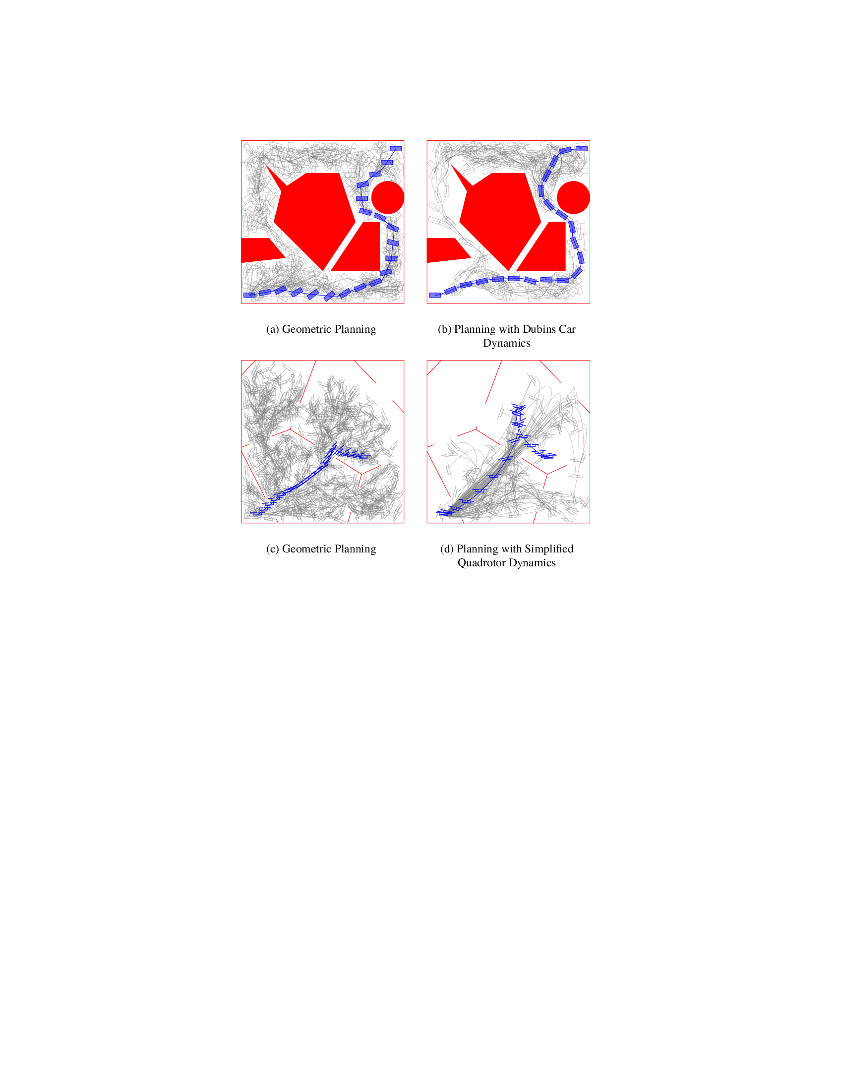
The geometric motion planning algorithms introduced so far assume no differential constraints on the robot’s motion. This assumption simplifies the planning task, as it allows the problem to be decomposed into two steps: first, computing a collision-free path that ignores dynamics, and then smoothing or reparameterizing this path so that it can be followed by the robot, as discussed in Chapter 3. However, purely geometric plans are not always straightforward to refine into dynamically feasible, optimized trajectories, often requiring downstream trajectory optimizers or controllers to perform aggressive corrections.

The kinodynamic motion planning problem extends geometric motion planning by explicitly accounting for a robot’s dynamics. Formally, let $\mathcal{X}\subseteq\mathbb{R}^{n}$ and $\mathcal{U}\subseteq\mathbb{R}^{m}$ denote the state and control spaces of a robotic system, respectively, and consider dynamics of the form:

\dot{\bm{x}}(t)\;=\;f(\bm{x}(t),\bm{u}(t)),\qquad\bm{x}(t)\in\mathcal{X},\;\bm% {u}(t)\in\mathcal{U}.

(4.7)

As in geometric planning, the robot’s configuration $q$ can be derived from the full dynamic state $\bm{x}$ , which encodes both position and the information needed for collision checking. The kinodynamic planning problem then seeks to drive the robot from an initial state $\bm{x}_{\mathrm{init}}$ to a goal region $\mathcal{X}_{\mathrm{goal}}$ while satisfying both collision avoidance and the system’s dynamical constraints.

By embedding kinematic and dynamic constraints at the planning stage, the planner produces nominal motions that are dynamically feasible by construction. This, in turn, provides better initializations for trajectory optimization and reduces the burden on the tracking controller, ultimately improving the overall system performance at execution time.

This formulation highlights the fundamental distinction between geometric and kinodynamic planning. In geometric planning, feasible paths are arbitrary collision-free curves in configuration space. In contrast, kinodynamic planning restricts admissible trajectories to those consistent with the system’s equations of motion. For example, a wheeled robot cannot move sideways, and a quadrotor cannot instantaneously stop due to inertia. These differential constraints drastically alter the search space, as illustrated in Figure 4.14, where adding dynamics constraints significantly restricts the feasible set of trajectories.

Forward-propagation-based algorithms.

A practical way to incorporate dynamics into sampling-based planners is through forward propagation. Rather than directly connecting sampled states, the planner samples a control input $\bm{u}\in\mathcal{U}$ and a duration $t$ , then integrates the system dynamics forward in time to produce a new state. For example, the kinodynamic extension of RRT proceeds by: (i) sampling a random state and finding its nearest neighbor $q_{\mathrm{near}}$ in the tree, (ii) sampling a random control $\bm{u}\in\mathcal{U}$ and propagation time $t$ , and (iii) simulating the system forward from $q_{\mathrm{near}}$ to obtain a new state. If the resulting trajectory segment is collision-free, it is added to the tree; otherwise, it is discarded. Notably, under mild regularity assumptions on $f(\bm{x}(t),\bm{u}(t))$ , variants of RRT with forward propagation have been shown to be probabilistically complete.

Kinodynamic planning thus unifies obstacle avoidance with differential constraints in a single framework, which is particularly important for robotics, where dynamical considerations highly restrict the set of feasible paths, for example in high-speed ground vehicles, aerial robots, or systems with significant momentum.

4.4.6 Should Probabilistic Planners be Probabilistic?

A natural question is whether the success of sampling-based algorithms depends fundamentally on the randomness of the sampling process. In particular, would the theoretical guarantees and practical performance of planners such as PRM^∗ or FMT^∗ still hold if the algorithms were de-randomized, i.e., run on deterministic samples?

This question is important for several reasons. Deterministic sampling sequences could substantially ease certification in safety-critical systems, since they remove probabilistic uncertainty. They would also allow planners to exploit offline computation more effectively, and simplify certain operations such as nearest-neighbor search.

Recent results show that the answer is affirmative, with carefully chosen low-dispersion deterministic sampling sequences, one can retain asymptotic optimality and completeness guarantees ²⁶26. Janson, L., Schmerling, E., Clark, A., Pavone, M. “Deterministic sampling-based motion planning: Optimality, complexity, and performance.” Int. Journal of Robotics Research 37(1), 46-61, 2018.. Thus, randomness is not strictly necessary for either correctness or performance. Probabilistic sampling provides convenience and generality, but deterministic low-dispersion sequences can yield equally strong guarantees while offering advantages in predictability, efficiency, and ease of certification.

4.5 Potential Field Methods

The planning methods described in the previous sections focus on capturing the global connectivity of the robot’s free space in a compact graph representation, which is then searched for a feasible path. In contrast, the approach introduced in this section is based on a fundamentally different idea. Potential field methods ²⁷27. Khatib, O. “Real-Time Obstacle Avoidance for Manipulators and Mobile Robots.” The International Journal of Robotics Research 5(1), 90-98, 1986. frame the motion planning problem using a physics-inspired analogy, where the robot is treated as a particle moving under the influence of an artificial potential field defined over the configuration space. This field is constructed to guide the robot toward its goal while simultaneously pushing it away from obstacles, resulting in a smooth, continuous path, as illustrated in Figure 4.15.

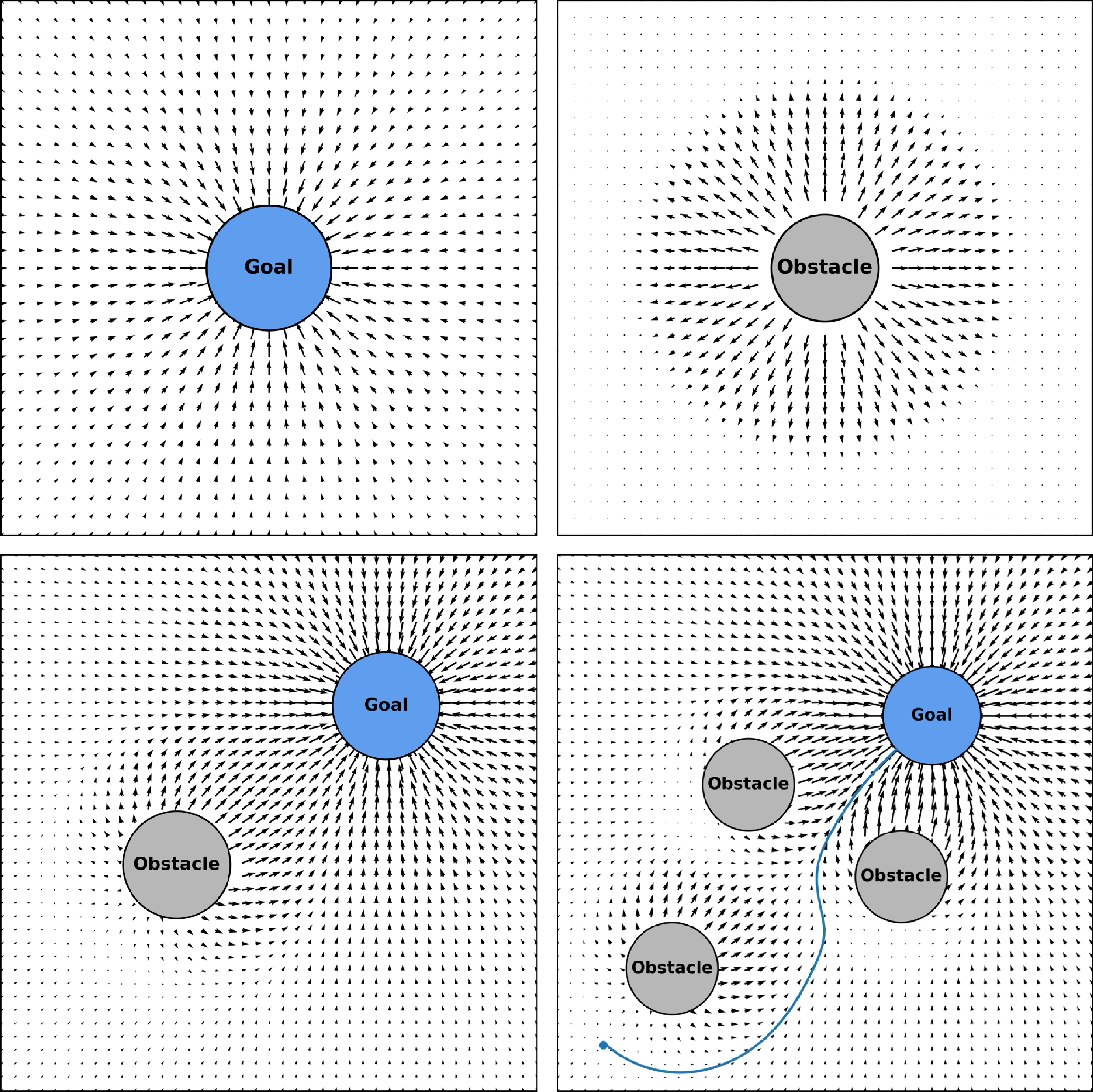
The core of this approach is the design of an artificial potential function $U(q):\mathcal{C}\to\mathbb{R}$ , which is typically composed of two components: an attractive potential $U_{\mathrm{att}}(q)$ that pulls the robot toward the goal configuration $q_{\mathrm{goal}}$ , and a repulsive potential $U_{\mathrm{rep}}(q)$ that pushes it away from obstacles:

U(q)=U_{\mathrm{att}}(q)+U_{\mathrm{rep}}(q).

(4.8)

The motion of the robot is then determined by following the negative gradient of this total potential $-\nabla U(q)$ , which represents the direction of steepest descent in the potential field. Specifically, the artificial force acting on the robot at configuration $q$ is given by:

\begin{split}F(q)=-\nabla U(q)&=-\nabla U_{\mathrm{att}}(q)-\nabla U_{\mathrm{% rep}}(q)\\ &=-F_{\mathrm{att}}(q)-F_{\mathrm{rep}}(q),\end{split}

(4.9)

where $F_{\mathrm{att}}(q)$ and $F_{\mathrm{rep}}(q)$ are the attractive and repulsive forces, respectively. A path is generated by starting at the initial configuration $q_{\mathrm{S}}$ and iteratively taking small steps in the direction of this force, effectively performing gradient descent on the potential surface until reaching the goal configuration $q_{\mathrm{G}}$ .

Below, we describe common choices for the attractive and repulsive potential functions and refer the reader to Latombe (1991)¹³13. Latombe, J. C. Robot Motion Planning. Kluwer Academic Publishers, 1991. for a more comprehensive treatment of potential field methods.

Attractive potential.

The attractive potential is designed to create a basin of attraction around the goal configuration—ideally, a unique global minimum—encouraging the robot to move toward it. A common choice for the attractive potential is a parabolic function of the form:

U_{\mathrm{att}}(q)=\frac{1}{2}k_{\mathrm{att}}\,\rho^{2}(q,q_{\mathrm{G}}),

(4.10)

where $k_{\mathrm{att}}$ is a positive scaling factor, and $\rho(q,q_{\mathrm{G}})$ denotes a distance metric (e.g., Euclidean distance) between the current configuration $q$ and the goal configuration $q_{\mathrm{G}}$ . The function $U_{\mathrm{att}}(q)$ is thus positive or null, and attains its minimum value at $q_{\mathrm{G}}$ , where $U_{\mathrm{att}}(q_{\mathrm{G}})=0$ .

The resulting attractive force (pointing toward the goal) is given by:

\begin{split}F_{\mathrm{att}}(q)&\coloneqq-\nabla U_{\mathrm{att}}(q)\\ &=-k_{\mathrm{att}}\,\rho(q,q_{\mathrm{G}})\nabla\rho(q,q_{\mathrm{G}})\\ &=-k_{\mathrm{att}}(q-q_{\mathrm{G}}),\\ &\text{where }\rho(q,q_{\mathrm{G}})=||q-q_{\mathrm{G}}||\text{ and }\nabla% \rho(q,q_{\mathrm{G}})=\frac{q-q_{\mathrm{G}}}{||q-q_{\mathrm{G}}||},\end{split}

(4.11)

which is a linear function of the distance to the goal.

Repulsive potential.

The repulsive potential is designed to create a potential barrier around obstacles, preventing the robot from colliding with them. Moreover, it should have a limited range of influence, affecting the robot only when it is within a certain distance from an obstacle. One way to achieve these properties is to define the repulsive potential as:

U_{\mathrm{rep}}(q)=\begin{cases}\frac{1}{2}k_{\mathrm{rep}}\left(\frac{1}{% \rho(q,\mathcal{C}_{\mathrm{obs}})}-\frac{1}{\rho_{0}}\right)^{2}&\text{if }% \rho(q,\mathcal{C}_{\mathrm{obs}})\leq\rho_{0},\\ 0&\text{if }\rho(q,\mathcal{C}_{\mathrm{obs}})>\rho_{0},\end{cases}

(4.12)

where $k_{\mathrm{rep}}$ is a positive scaling factor, $\rho(q,\mathcal{C}_{\mathrm{obs}})$ denotes the distance from the configuration $q$ to the nearest obstacle in the configuration space, and $\rho_{0}$ is a threshold distance beyond which the repulsive potential has no effect, also referred to as the distance of influence. Formally, the distance to the nearest obstacle is defined as:

\rho(q,\mathcal{C}_{\mathrm{obs}})=\min_{q^{\prime}\in\mathcal{C}_{\mathrm{obs% }}}\rho(q,q^{\prime}),

(4.13)

where $\mathcal{C}_{\mathrm{obs}}$ is the set of configurations that result in collisions with obstacles.

If $\mathcal{C}_{\mathrm{obs}}$ is a convex region, $\rho(q,\mathcal{C}_{\mathrm{obs}})$ is differentiable everywhere in $\mathcal{C}_{\mathrm{free}}$ , and the resulting repulsive force is given by:

\begin{split}F_{\mathrm{rep}}(q)&\coloneqq-\nabla U_{\mathrm{rep}}(q)\\ &=\begin{cases}k_{\mathrm{rep}}\left(\frac{1}{\rho(q,\mathcal{C}_{\mathrm{obs}% })}-\frac{1}{\rho_{0}}\right)\frac{1}{\rho^{2}(q,\mathcal{C}_{\mathrm{obs}})}% \nabla\rho(q,\mathcal{C}_{\mathrm{obs}})&\text{if }\rho(q,\mathcal{C}_{\mathrm% {obs}})\leq\rho_{0},\\ 0&\text{if }\rho(q,\mathcal{C}_{\mathrm{obs}})>\rho_{0}.\end{cases}\end{split}

(4.14)

Specifically, let $q_{\mathrm{obs}}^{\ast}$ be the point on the boundary of the obstacle closest to $q$ , i.e., $q_{\mathrm{obs}}^{\ast}=\arg\min_{q^{\prime}\in\mathcal{C}_{\mathrm{obs}}}\rho% (q,q^{\prime})$ . Then, the gradient $\nabla\rho(q,\mathcal{C}_{\mathrm{obs}})$ is a unit vector pointing away from $\mathcal{C}_{\mathrm{obs}}$ and supported by the line segment connecting $q_{\mathrm{obs}}^{\ast}$ to $q$ .

Advantages and disadvantages.

The primary advantage of potential field methods is their simplicity and computational efficiency. These methods were originally developed as an online collision avoidance strategy for mobile robots²⁸28. Khatib, O. “Real-Time Obstacle Avoidance for Manipulators and Mobile Robots.” The International Journal of Robotics Research 5(1), 90-98, 1986., applicable in dynamic environments where obstacles may not be known in advance. Instead of performing a complex search over a graph or constructing a roadmap, path generation simply involves evaluating the potential function and its gradient at the robot’s current configuration.

However, since potential field planners essentially act as gradient descent algorithms on the potential function, they are susceptible to local minima. Specifically, the planner can become trapped in regions where the attractive and repulsive forces balance out, resulting in a net force of zero at a configuration that is not the goal. This issue commonly occurs in environments with concave obstacles (e.g., a U-shaped trap) or in narrow corridors where the repulsive forces from opposing walls can cancel the attractive pull toward the goal. Because of this, standard potential field planners are not complete and may fail to find a path even when one exists.

Several techniques have been proposed to address the local minima problem. One approach is to introduce a random “jiggle” (e.g., a small random perturbation to the robot’s configuration) to escape the basin of a local minimum. A more theoretically grounded solution involves constructing special potential fields called navigation functions, which are provably free of local minima except for the goal ²⁹29. Rimon, E. Exact robot navigation using artificial potential functions. PhD Thesis. Yale University, 1990.. However, constructing such functions is computationally expensive and generally only feasible for simple environments. Another related approach, the wavefront planner or brushfire algorithm, discretizes the configuration space (similar to grid-based methods) and propagates a potential wave outward from the goal, effectively creating a potential field on a grid that is guaranteed to be free of local minima.

In summary, potential field methods provide a fast and reactive framework for local motion planning and obstacle avoidance. While their simplicity is appealing, their unreliability for global planning due to the local minima problem limits their use as a standalone, complete motion planner.

4.6 Summary

In this chapter, we introduced motion planning as the critical link that translates high-level task specifications into feasible, collision-free paths. We formulated the core problem as finding a sequence of actions that drives a robot from a start configuration to a goal configuration while avoiding obstacles. A central theme was the abstraction of motion into the robot’s configuration space ( $\mathcal{C}$ -space), where planning reduces to finding a continuous path in the free space, $\mathcal{C}_{\mathrm{free}}$ .

We began by discussing grid-based methods, which discretize the configuration space and cast the problem as a shortest-path search on a graph. This allowed us to introduce a general family of label-correcting algorithms, including Dijkstra’s algorithm for finding shortest paths, and its informed extension, A*, which uses heuristics to guide the search efficiently toward the goal. We then turned to combinatorial planning, an exact approach that constructs a roadmap by decomposing the continuous free space into simple cells, guaranteeing completeness but facing computational challenges in high-dimensional spaces. Next, we discussed sampling-based methods, which avoid the explicit construction of the free space by relying on random sampling and collision detection to incrementally build $\mathcal{C}_{\mathrm{free}}$ . We presented the PRM algorithm, a multi-query planner that builds a reusable graph of the free space, and the single-query RRT algorithm, which incrementally grows a tree from the start configuration. We summarized their key theoretical properties, including probabilistic completeness and asymptotic optimality, which motivated advanced planners like PRM*, RRT* and the FMT* algorithm. We further extended these concepts to kinodynamic planning, which incorporates system dynamics, and discussed how deterministic low-dispersion sampling can provide similar theoretical guarantees as probabilistic methods while offering benefits in predictability and certification. Finally, we introduced potential field methods, which generate paths by defining artificial potential functions that attract the robot to the goal while repelling it from obstacles, enabling fast and reactive local planning at the cost of potential local minima.

To learn more.

For a deeper exploration of the topics covered in this chapter, several key resources are available. For a comprehensive and foundational treatment of motion planning, from configuration spaces to combinatorial and sampling-based algorithms, the textbook by LaValle (2006)¹⁴14. LaValle, S. M. Planning Algorithms. Cambridge University Press, 2006. is an essential reference. An in-depth presentation of grid-based planning methods and shortest path algorithms is provided in Bertsekas (2000)¹⁵15. Bertsekas, D. Dynamic Programming and Optimal Control. Athena Scientific, 2000.. A detailed treatment of the D* algorithm for planning in dynamic environments can be found in Stentz (1995)¹⁶16. Stentz, A. “The focussed D* algorithm for real-time replanning.” In 14th International Joint Conference on Artificial Intelligence, 1652–1659, 1995.. The seminal work on asymptotic optimality for sampling-based planners, which introduced PRM* and RRT*, is presented in Karaman and Frazzoli (2011)¹⁷17. Karaman, S., Frazzoli, E. “Sampling-based Algorithms for Optimal Motion Planning.” Int. Journal of Robotics Research 30(7), 846–894, 2011.. For an in-depth discussion of the FMT* algorithm, we refer the reader to Janson et al. (2015)¹⁸18. Janson, L., Schmerling, E., Clark, A., Pavone, M. “Fast Marching Tree: A Fast Marching Sampling-Based Method for Optimal Motion Planning in Many Dimensions.” Int. Journal of Robotics Research 34(7), 883–921, 2015.. Kinodynamic planning is thoroughly discussed in Schmerling and Pavone (2019)¹⁹19. Schmerling, E., Pavone, M. “Kinodynamic Planning.” In Encyclopedia of Robotics. Springer, 2019.. The extension of performance guarantees to deterministic sampling patterns is explored in Janson et al. (2018)²⁰20. Janson, L., Schmerling, E., Clark, A., Pavone, M. “Deterministic sampling-based motion planning: Optimality, complexity, and performance.” Int. Journal of Robotics Research 37(1), 46-61, 2018.. The original formulation of potential field methods for robot motion planning was introduced by Khatib (1986)²¹21. Khatib, O. “Real-Time Obstacle Avoidance for Manipulators and Mobile Robots.” The International Journal of Robotics Research 5(1), 90-98, 1986., and a comprehensive discussion can be found in Latombe (1991)²²22. Latombe, J. C. Robot Motion Planning. Kluwer Academic Publishers, 1991.. Finally, for a more modern review of motion planning techniques and their applications in robotics, we recommend the survey by Hauser (2020)²³23. Hauser, K. “Motion and Path Planning.” In Encyclopedia of Robotics, 1–11. Springer, 2020..

4.7 Exercises

The starter code for the exercises provided below is available online through GitHub. To get started, download the code by running in a terminal window:

⬇

git clone https://github.com/StanfordASL/pora-exercises.git

We denote Problems requiring hand-written solutions and coding in Python with and , respectively.

Problem 1: A* motion planning

In this exercise, you will implement the A* grid-based motion planning algorithm for some simple two-dimensional environments. In the files
ch04/exercises/a_star.ipynb and ch04/exercises/a_star.py, you will implement the key parts of the A* algorithm (see Algorithm 2), run the algorithm on some randomly generated path planning problems, and then explore a way to smooth the resulting discrete paths, which could be useful for practical robot motion planning tasks.

Data: Start node

q_{\mathrm{S}}

, goal node

q_{\mathrm{G}}

Result: Shortest path from

q_{\mathrm{S}}

q_{\mathrm{G}}

(if reachable)

\mathcal{O}\leftarrow\{q_{\mathrm{S}}\}

/* Initialize open set */

\mathcal{C}\leftarrow\{\}

/* Initialize closed set */

C(q_{\mathrm{S}})\leftarrow 0

/* Initialize cost-to-arrive */

\tilde{C}(q_{\mathrm{S}})\leftarrow\mathsf{distance}(q_{\mathrm{S}},q_{\mathrm%{G}})

/* Initialize estimated cost */

while $\mathcal{O}$ is not empty do

q\leftarrow\mathsf{lowest\_est\_cost\_through}(\mathcal{O})

if $q=q_{\mathrm{G}}$ then

return $\mathrm{reconstruct\_path}()$

\mathcal{O}.\mathrm{remove}(q)

\mathcal{C}.\mathrm{add}(q)

for $q^{\prime}\in\mathrm{free\_neighbors}(q)$ do

if $q^{\prime}\in\mathcal{C}$ then

continue

if $q^{\prime}\not\in\mathcal{O}$ then

\mathcal{O}.\mathrm{add}(q^{\prime})

else if $C(q)+\mathsf{distance}(q,q^{\prime})>C(q^{\prime})$ then

continue

\mathrm{parent}(q^{\prime})\leftarrow q

C(q^{\prime})\leftarrow C(q)+\mathsf{distance}(q,q^{\prime})

\tilde{C}(q^{\prime})\leftarrow C(q^{\prime})+\mathsf{distance}(q^{\prime},q_{%\mathrm{G}})

return $\mathrm{Failure}$

Algorithm 2 A* Motion Planning

In this implementation of A*, we will represent the free space by a graph, which is traversed by sampling and collision-checking states from a deterministic grid. This implementation can be categorized as informed, deterministic sampling-based planning (“informed” due to the A* heuristic).

1.
Implement the remaining functions in a_star.py within the Astar class. These functions represent many of the key functional blocks at play in motion planning algorithms:
- •
  
  is_free which checks whether a state is collision-free and valid.
- •
  
  distance which computes the travel distance between two points.
- •
  
  get_neighbors which finds the free neighbor states of a given state.
- •
  
  solve which runs the A* motion planning algorithm.

Note: Notice that we collision-check states but do not collision-check edges. This saves us some computation (collision-checking is often one of the most expensive operations in motion planning). Also, in this case the obstacles are aligned with the grid, so paths will remain collision-free. However, outside such special circumstances we should add edge collision-checking and/or inflate obstacles to guarantee collision-avoidance.

2.

Planning a path on a grid is often not very desirable for a real robot that would have to track the trajectory. In this exercise, we will smooth the paths from A* by fitting a cubic spline to the path nodes. Implement this within the compute_smooth_plan function of a_star.ipynb.

Note: There are many ways to ensure smoothed solutions are collision-free (for example, collision-checking smoothed paths and running a dichotomic search on the smoothing parameters to find a tight fit against obstacles, or inflating obstacles in the original planning to give additional room for smoothing). This strategy can be used on geometric sampling-based planning methods as well.

Problem 2: Rapidly-exploring random trees

In this exercise, you will implement the RRT sample-based motion planning algorithm to plan paths in simple 2D environments. In the files
ch04/exercises/rrt.ipynb and ch04/exercises/rrt.py, you will implement the key parts of the RRT algorithm and define a GeometricRRT planner that leverages simple straight line connections between nodes.

For this implementation of RRT, we consider a “Geometric” RRT problem where nodes are connected with simple straight lines.

Data: Start node

q_{\mathrm{S}}

, goal node

q_{\mathrm{G}}

, max iterations

N_{\max}

, goal sampling bias

\alpha

Result: Path from

q_{\mathrm{S}}

q_{\mathrm{G}}

(if reachable)

\mathcal{T}\leftarrow\{q_{\mathrm{S}}\}

/* Initialize tree */

for $k\leftarrow 1$ to $N_{\max}$ do

if $\mathrm{rand()}<\alpha$ then

q^{\prime}\leftarrow q_{\mathrm{G}}

else

q^{\prime}\leftarrow\mathrm{random\_sample()}

q\leftarrow\mathrm{nearest\_neighbor}(q^{\prime},\mathcal{T})

q^{\prime}\leftarrow\mathrm{steer\_towards}(q,q^{\prime})

if $\mathrm{is\_free\_motion}(q,q^{\prime})$ then

\mathrm{parent}(q^{\prime})\leftarrow q

\mathcal{T}.\mathrm{add}(q^{\prime})

if $q^{\prime}=q_{\mathrm{G}}$ then

return $\mathrm{reconstruct\_path}()$

return $\mathrm{Failure}$

Algorithm 3 RRT Motion Planning

1.
Implement the remaining functions in rrt.py within the RRT and GeometricRRT classes:
- •
  
  RRT.solve which runs the RRT algorithm in Algorithm 3.
- •
  
  GeometricRRT.nearest_neighbor which computes the nearest neighbor in the current tree to a given point using Euclidean distance.
- •
  
  GeometricRRT.steer_towards to compute a new state from a target state following a straight line path.
2.

Implement the function RRT.shortcut_path to try to find a shorter path from the existing tree by removing nodes from the path that aren’t strictly needed. Run the code in rrt.ipynb to check your work.
3.

Run the provided code (RRT.solve_optimal) to compare the standard RRT algorithm you implemented against the RRT* algorithm.

4.1 Problem Formulation

Example 4.1.1 (L-shaped Robot).

Free space in configuration space.

4.2 Grid-based Motion Planning

Connectivity and neighborhood structure.

4.2.1 Label Correcting Algorithms

General structure of label-correcting algorithms.

The role of the selection rule.

Beyond Dijkstra: toward more informed search for motion planning.

Theorem 4.1 (Correctness of a graph search algorithm; Bertsekas (2000)22. Bertsekas, D. Dynamic Programming and Optimal Control. Athena Scientific, 2000.).

The A* algorithm.

The D* algorithm.

Pros and cons of grid-based planning.

4.3 Combinatorial Motion Planning

The roadmap.

4.3.1 Cell Decomposition

Vertical cell decomposition.

Example 4.3.1 (2D Cell Decomposition).

4.3.2 Other Roadmap Construction Methods

4.4 Sampling-based Motion Planning

4.4.1 Probabilistic Roadmaps (PRMs)

Design considerations.

Characteristics of PRMs.

4.4.2 Rapidly-Exploring Random Trees (RRTs)

Voronoi bias.

4.4.3 Theoretical Guarantees

Probabilistic completeness.

Asymptotic optimality.

Theorem 4.1.

Example 4.4.1 (PRM* in 2D Workspace).

4.4.4 Fast Marching Tree Algorithm (FMT∗)

High-level description.

4.4.5 Kinodynamic Planning

Forward-propagation-based algorithms.

4.4.6 Should Probabilistic Planners be Probabilistic?

4.5 Potential Field Methods

Attractive potential.

Repulsive potential.

Advantages and disadvantages.

4.6 Summary

To learn more.

4.7 Exercises

Problem 1: A* motion planning

Problem 2: Rapidly-exploring random trees

Practice · 3 notebooks

Theorem 4.1 (Correctness of a graph search algorithm; Bertsekas (2000)²2. Bertsekas, D. Dynamic Programming and Optimal Control. Athena Scientific, 2000.).

4.4.4 Fast Marching Tree Algorithm (FMT^∗)