Open-Loop Control & Trajectory Optimization

In Chapter 1, we introduced the state space model as a mathematical formulation for representing a robot’s dynamics. These models, typically expressed as systems of differential equations, provide a foundational framework that describes how the state of a robot evolves over time in response to control inputs. In particular, we saw how a state space model can be derived from the robot’s kinematics and dynamics, providing a compact yet expressive description of its physical motion. In this chapter, we turn to a fundamental question: given a state space model of the robot, how can we determine the control inputs that will drive it to execute a desired behavior?

As we will see throughout Chapters Chapter 2-Chapter 4, robots must transform high-level goals into precise physical actions. This process is often described hierarchically, spanning decision-making, motion planning, trajectory optimization, and control (Figure 2.1). Each layer plays a distinct role, yet they remain deeply interconnected.

At the higher level of this hierarchy, decision-making governs what tasks the robot should perform to fulfill its objectives. It involves reasoning over goals, resources, and constraints, often under uncertainty. In a self-driving car, for example, this may correspond to deciding when to overtake, yield, or reroute. Because it involves strategic considerations rather than immediate actuation, decision-making typically unfolds on the order of seconds to minutes. Ultimately, decision-making defines the high-level objectives that guide subsequent layers of the hierarchy.

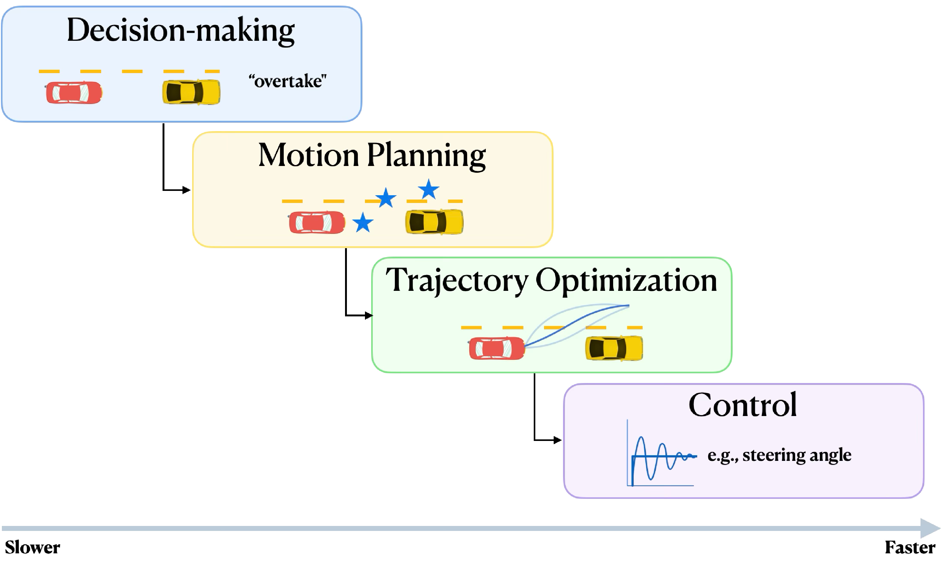
Refer to caption — Figure 2.1: A hierarchical view of the relationship between decision-making, motion planning, trajectory optimization, and control.

Once a high-level decision has been made, motion planning determines how to realize it in the robot’s physical environment. This is typically expressed in terms of the robot’s configuration space and involves finding a collision-free path that respects geometric and kinematic constraints. For instance, motion planning may compute a path for a mobile robot to navigate a cluttered warehouse without collisions. The timescale of motion planning is often on the order of hundreds of milliseconds to seconds.

Building on this path, trajectory optimization refines it into a time-parameterized trajectory that is dynamically feasible and optimized for performance criteria. This entails solving continuous optimization problems that incorporate dynamics, actuator limits, and objectives such as energy efficiency, comfort, or safety margins. The result is a trajectory specifying both the robot’s states and the control inputs needed to realize them over time, ensuring compatibility with the robot’s actuation capabilities and dynamic constraints. Trajectory optimization typically operates on shorter timescales, from tens to hundreds of milliseconds.

Finally, low-level control ensures that the robot faithfully executes the desired trajectory in the physical world, by converting the trajectory into actuation commands. Controllers must operate at high frequency, applying feedback to correct deviations caused by disturbances, modeling errors, or sensor noise. Whether adjusting wheel torques, joint forces, or thrust vectors, control is what closes the loop between higher-level plans and physical reality.

Together, these layers form the backbone of an autonomous system: decision-making provides strategic guidance, motion planning translates that guidance into feasible paths, trajectory optimization refines those paths into feasible and optimal trajectories, and control ensures that the robot can follow those trajectories in the real world. In practice, the boundaries between these layers are often blurred. Trajectory optimization, for instance, may be tightly integrated with planning or even embedded within control loops, while high-level decisions may be informed by the lower-level processes. For the purposes of this book, we will adopt the hierarchical perspective outlined above, while acknowledging that real-world systems frequently combine or intertwine these processes.

In this chapter, we focus on trajectory optimization as a fundamental tool for computing trajectories that are both feasible and optimal. While control and motion planning will be revisited in Chapter Chapter 3 and Chapter Chapter 4, respectively, our emphasis in this chapter is on the formulation and solution of the trajectory optimization problem. We begin in Section 2.1 by introducing the trajectory optimization problem and casting it as a continuous optimization problem. Building on this foundation, Sections 2.2 and Section 2.3 present two major classes of solution strategies—indirect methods, which derive optimality conditions for the continuous problem using tools from the calculus of variations, and direct methods, which discretize and numerically solve the problem as a finite-dimensional nonlinear program. Finally, in Section 2.4, we explore specialized techniques tailored to certain problem structures, known as differentially flat systems.

2.1 The Optimal Control Problem

Optimal control theory aims to determine control inputs that drive a dynamical system to satisfy its physical constraints while optimizing a performance criterion. At a high level, formulating an optimal control problem requires three key components:

•

A mathematical model of the system, typically expressed in state space form.
•

A description of the physical constraints the system must satisfy.
•

A specification of the performance criterion to be optimized.

Mathematical model.

As discussed extensively in Chapter 1, the purpose of a mathematical model is to describe how the system’s state evolves over time in response to control inputs. Using the notation from Chapter 1, the system dynamics can be expressed as a set of ordinary differential equations:

\dot{\bm{x}}(t)=f\left(\bm{x}(t),\bm{u}(t)\right),

(2.1)

where $\bm{x}(t)\in\mathbb{R}^{n}$ is the state of the system at time $t$ , $\bm{u}(t)\in\mathbb{R}^{m}$ is the control input, and $f:\mathbb{R}^{n}\times\mathbb{R}^{m}\to\mathbb{R}^{n}$ defines the state evolution over time. Throughout this book, we will often refer to $\bm{x}(t)$ and $\bm{u}(t)$ as the state and control sequences, respectively, or equivalently as the state and control trajectories.

Physical constraints.

Once we define the system dynamics, the next step is to specify the physical constraints that the system must satisfy. These constraints can take several forms, including:

•

Initial conditions, which specify the state at the initial time $t_{0}$ as $\bm{x}(t_{0})=\bm{x}_{0}$ .
•

Final conditions, which specify the state at the final time $t_{f}$ as $\bm{x}(t_{f})=\bm{x}_{f}$ or $\bm{x}(t_{f})\in\mathcal{X}_{f}$ , where $\mathcal{X}_{f}$ denotes a set of allowable terminal states.
•

State constraints, which require that the state remains within an allowable set $\mathcal{X}$ for all times $t\in[t_{0},t_{f}]$ , that is, $\bm{x}(t)\in\mathcal{X}$ .
•

Control constraints, which enforce that the control input remains within an allowable set $\mathcal{U}$ for all times $t\in[t_{0},t_{f}]$ , that is, $\bm{u}(t)\in\mathcal{U}$ .

Depending on whether the constraints are satisfied or not, we can define the concept of admissibility for a control history and state trajectory.

Definition 2.1 (Admissible State and Control Sequences).

A state trajectory $\bm{x}(t)$ and a control sequence $\bm{u}(t)$ are admissible if they satisfy the state and control constraints at all times, that is:

\bm{x}(t)\in\mathcal{X}\quad\text{and}\quad\bm{u}(t)\in\mathcal{U},\quad% \forall t\in[t_{0},t_{f}].

Admissibility is a key concept in optimal control, as it restricts the set of realizable trajectories^†^†margin: In practice, this allows numerical methods to focus exclusively on admissible state and control sequences, rather than considering all possible solutions. .

Performance criterion.

The final component of an optimal control problem is the performance criterion to be optimized. An optimal control is defined as one that minimizes (or maximizes) this performance criterion. In some cases, the performance criterion may be implicitly defined by the problem statement (e.g., minimizing the time to reach a goal state), whereas in other cases, it must be explicitly designed (e.g., driving a car in a way that is comfortable for the passengers).

Throughout this book, we will focus on performance criteria that can be expressed as a cost functional^†^†margin: A functional maps functions to real numbers; intuitively, we might say that a functional is a “function over functions”. Here, the cost functional maps a state trajectory and control sequence to a real number representing the overall cost. of the form:

J(\bm{x}(t),\bm{u}(t),t)=h(\bm{x}(t_{f}),t_{f})+\int_{t_{0}}^{t_{f}}g(\bm{x}(t% ),\bm{u}(t),t)\,dt,

(2.2)

where $h:\mathbb{R}^{n}\times\mathbb{R}\to\mathbb{R}$ is the terminal cost and $g:\mathbb{R}^{n}\times\mathbb{R}^{m}\times\mathbb{R}\to\mathbb{R}$ is the running cost. The terminal cost $h$ is evaluated at the final time $t_{f}$ and typically represents a cost associated with the state of the system at that time, such as a penalty for being far from a desired goal state. The running cost $g$ is integrated over the time interval $[t_{0},t_{f}]$ and represents the instantaneous cost incurred by the system at each time step, for example, the cost of energy consumption, or any other cost associated with the system’s operation. Depending on the problem, the final time $t_{f}$ may be finite and fixed, finite and free, or infinite^†^†margin: In the case of an infinite final time, the terminal cost $h$ is typically ignored and set to zero. .

2.1.1 Problem Formulation

As a result, an optimal control problem can be formulated as follows:

Determine an admissible control sequence $\bm{u}^{*}(t)$ such that the system dynamics:

\dot{\bm{x}}(t)=f(\bm{x}(t),\bm{u}(t),t),

generate a corresponding admissible state trajectory $\bm{x}^{*}(t)$ that minimizes the performance criterion:

J(\bm{x}(t),\bm{u}(t),t)=h(\bm{x}(t_{f}),t_{f})+\int_{t_{0}}^{t_{f}}g(\bm{x}(t% ),\bm{u}(t),t)\,dt,

where $\bm{u}^{*}(t)$ and $\bm{x}^{*}(t)$ are referred to as the optimal control sequence and optimal state trajectory, respectively.

This problem can be formally posed as the following optimization problem:

$\displaystyle\underset{\bm{u}(t)}{\text{minimize}}$	$\displaystyle J(\bm{x}(t),\bm{u}(t),t),$	(2.3)
subject to	$\displaystyle\dot{\bm{x}}(t)=f(\bm{x}(t),\bm{u}(t),t),$
	$\displaystyle\bm{x}(t_{0})=\bm{x}_{0},\quad\bm{x}(t_{f})=\bm{x}_{f},$
	$\displaystyle\bm{u}(t)\in\mathcal{U},\quad\bm{x}(t)\in\mathcal{X},\quad t_{0}<% t<t_{f}.$

This general formulation serves as the starting point for the optimal control methods developed in the remainder of this book. There are also several important attributes related to the solution of this problem that are worth highlighting:

1.

Existence: A solution to an optimal control problem is not guaranteed to exist; there may be no control history that is both admissible and optimal.
2.

Uniqueness: Even when a solution exists, it may not be unique. Multiple admissible control inputs can yield the same performance. While this can pose challenges for numerical algorithms, it also provides flexibility in selecting among equally good solutions depending on the application.
3.

Optimality: The objective of optimal control is to find a control sequence that outperforms all other admissible candidates. Thus, optimal control is interested in global optimality, as opposed to local optimality.

Example 2.1.1 (Autonomous Racing Optimal Control).

Consider an autonomous racing scenario in which the goal is to complete a lap of a known course in the shortest possible time. We can formulate this as a finite-horizon optimal control problem, where the objective is to minimize the final time $t_{f}$ required to reach a designated goal position $(x_{\text{goal}},y_{\text{goal}})$ , subject to the constraint that the vehicle must remain on the track at all times. Let $\mathcal{X}_{\mathbb{course}}$ denote the set of admissible states that correspond to positions on the course.

Suppose the vehicle is modeled using the simple kinematic car model from Equation 1.29, with state $\bm{x}=\left[{x,\>y,\>\theta}\right]^{\top}$ representing position and heading, and control inputs $\bm{u}=\left[{v,\>\phi}\right]^{\top}$ representing forward speed and steering angle, respectively. The resulting optimal control problem is:

	$\displaystyle\underset{v(t),\,\phi(t)}{\text{minimize}}$	$\displaystyle t_{f},$
	subject to	$\displaystyle\dot{x}=v\cos\theta,\quad\dot{y}=v\sin\theta,\quad\dot{\theta}=% \frac{v}{L}\tan\phi,$
		$\displaystyle\bm{x}\in\mathcal{X}_{\text{course}},\quad\bm{u}\in\mathcal{U},$
		$\displaystyle\bm{x}(t_{0})=\bm{x}_{0},\quad(x(t_{f}),y(t_{f}))=(x_{\text{goal}% },y_{\text{goal}}).$

In this formulation, the cost depends only on the final time and not directly on the state or control at intermediate points. As a result, the time-optimal solution $(\bm{x}(t),\bm{u}(t))$ will lie on the boundaries of the admissible control and state sets. In practice, this means the vehicle will operate at full throttle and steer at the physical limits to cut the lap time, a strategy that achieves optimality mathematically—but may not make for a smooth or comfortable ride.

Throughout this book, we will see that the solution to the optimal control problem can take different forms, depending on whether and how it incorporates feedback from the current state of the system. At the most fundamental level, we distinguish between open-loop and closed-loop control. While closed-loop control will be the focus of Chapter 3, this chapter addresses open-loop control.

Open-loop control.

If the optimal control is computed purely as a function of time for a given initial state,

\bm{u}^{*}(t)=\ell(\bm{x}(t_{0}),t),

(2.4)

it is said to be in open-loop form. In the context of trajectory optimization, restricting the focus to open-loop strategies is natural, as they balance computational efficiency—computing open-loop sequences is faster than computing closed-loop policies—with effectiveness, since robustness can be endowed through closed-loop tracking or by re-optimizing the trajectory in a receding-horizon fashion, as in Model Predictive Control^†^†margin: Discussed further in Chapter 3. .

Having introduced the optimal control problem, we now turn to methods for computing optimal open-loop solutions. Fundamentally, Problem (Equation 2.3) is an infinite-dimensional optimization problem, where the optimization variables are functions of time. In practice, solution methods must rely on discretization strategies, thereby approximating the infinite-dimensional problem with a finite-dimensional one. Different discretization approaches give rise to distinct families of methods.

Broadly speaking, two main classes of methods exist: indirect methods and direct methods. Indirect methods follow an “optimize-then-discretize” paradigm: they first derive necessary conditions for optimality—typically in the form of boundary-value problems involving adjoint variables—and then apply numerical techniques to solve these conditions. In contrast, direct methods take a “discretize-then-optimize” approach: the state and control sequences are parameterized using finite-dimensional representations, and the resulting finite-dimensional optimization problem is solved numerically.

Beyond these two general classes, some systems admit further structural simplifications. In particular, differentially flat systems allow trajectories to be described in terms of a small set of variables that fully capture the system’s evolution^†^†margin: These variables are commonly known as flat outputs. . This property enables efficient trajectory generation and optimization, making these systems especially relevant in mobile robotics and aerospace applications.

The remainder of this chapter examines these three classes of methods in detail: indirect methods in Section 2.2, direct methods in Section 2.3, and trajectory optimization for differentially flat systems in Section 2.4.

2.2 Indirect Methods

Indirect methods provide a principled framework for solving optimal control problems by drawing on ideas from calculus of variations (CoV)^†^†margin: Calculus of variations extends the principles of classical calculus from functions to functionals. The central idea is to study how small perturbations—called variations—of a candidate function influence the value of the functional. By analyzing the first- and higher-order effects of these variations, one can derive necessary conditions for optimality. . For a comprehensive treatment of the calculus of variations and its applications in optimal control theory, we refer the reader to Kirk (2004)¹1. Kirk, D. E. Optimal Control Theory: An Introduction. Dover Publications, 2004.. At their core, indirect methods rely on the derivation of necessary optimality conditions (NOCs) that any solution must satisfy and then leverage numerical techniques to compute solutions consistent with these conditions. In this way, the NOCs serve as the bridge between the continuous-time formulation of an optimal control problem and its numerical resolution.

Before turning to the derivation of such conditions for infinite-dimensional optimization problems, let us first review key concepts from finite-dimensional optimization, which will serve as a foundation for the discussion ahead.

2.2.1 NOCs for Unconstrained Nonlinear Optimization Problems

Consider the following finite-dimensional optimization problem:

\underset{[}{\text{minimize}}\>\quad\bm{x}\in\mathbb{R}^{n}]f(\bm{x}),

(2.5)

where $f:\mathbb{R}^{n}\to\mathbb{R}$ is assumed continuously differentiable, i.e., $f\in C^{1}$ . We wish to identify the NOCs that any minimizer—local or global—must satisfy.

The key intuition is that at a local minimizer, no infinitesimal perturbation of the decision variable should decrease the objective. Formally, this requires analyzing how $f$ changes under small variations around a candidate minimizer $\bm{x}^{*}$ .

First-order necessary condition.

Let $\bm{x}^{*}\in\mathbb{R}^{n}$ be a local minimizer. If $f\in C^{1}$ , we can use gradients and Taylor series expansions to characterize the behavior of $f$ near $\bm{x}^{*}$ . For a small perturbation $\Delta x$ , the cost variation is, up to first order:

f(\bm{x}^{*}+\Delta x)-f(\bm{x}^{*})\approx\nabla f(\bm{x}^{*})^{\top}\Delta x.

If $\bm{x}^{*}$ is a local minimizer, then for sufficiently small $\Delta x$ , the first-order term must be non-negative^†^†margin: This is because, if we were to decrease the cost by perturbing $\bm{x}^{*}$ by $\Delta x$ , then $\bm{x}^{*}$ would not be a local minimizer. :

\nabla f(\bm{x}^{*})^{\top}\Delta x=\sum_{i=1}^{n}\frac{\partial f(\bm{x}^{*})% }{\partial x_{i}}\Delta x_{i}\geq 0.

In particular, by taking $\Delta\bm{x}$ to be positive and negative multiples of the coordinate unit vectors, that is, vectors having all components equal to zero except for one component equal to one, we obtain simultaneously:

\frac{\partial f(\bm{x}^{*})}{\partial x_{i}}\geq 0\quad\text{and}\quad\frac{% \partial f(\bm{x}^{*})}{\partial x_{i}}\leq 0,\qquad i=1,\ldots,n,

which forces the condition:

\frac{\partial f(\bm{x}^{*})}{\partial x_{i}}=0,\qquad i=1,\ldots,n,

or, more compactly:

\nabla f(\bm{x}^{*})=0.

Thus, any local minimizer $\bm{x}^{*}$ must be a stationary point of $f$ .

Second-order necessary condition.

Assuming $f\in C^{2}$ , consider again the Taylor expansion of $f$ around a local minimizer $\bm{x}^{*}$ , this time up to second order:

f(\bm{x}^{*}+\Delta x)-f(\bm{x}^{*})\approx\nabla f(\bm{x}^{*})^{\top}\Delta x% +\frac{1}{2}\Delta x^{\top}\nabla^{2}f(\bm{x}^{*})\Delta x.

For $\bm{x}^{*}$ to be a local minimizer, the second-order variation must be nonnegative for all sufficiently small $\Delta\bm{x}$ , that is:

\nabla f(\bm{x}^{*})^{\top}\Delta x+\frac{1}{2}\Delta x^{\top}\nabla^{2}f(\bm{% x}^{*})\Delta x\geq 0.

Using the first-order condition $\nabla f(\bm{x}^{*})=0$ , the linear term vanishes, leaving:

\Delta x^{\top}\nabla^{2}f(\bm{x}^{*})\Delta x\geq 0.

Thus, the Hessian $\nabla^{2}f(\bm{x}^{*})$ must be positive semidefinite at any local minimizer.

Theorem 2.1 (Necessary Conditions for Unconstrained Local Minimizers).

Let $\bm{x}^{*}$ be a local minimizer of $f:\mathbb{R}^{n}\to\mathbb{R}$ . If $f\in C^{1}$ in an open set containing $\bm{x}^{*}$ , then:

\nabla f(\bm{x}^{*})=0\quad\text{(first-order NOC)}.

(2.6)

If, in addition, $f\in C^{2}$ , then:

\nabla^{2}f(\bm{x}^{*})\succeq 0\quad\text{(second-order NOC)}.

(2.7)

2.2.2 NOCs for Constrained Nonlinear Optimization Problems

Having introduced the NOCs for unconstrained problems, this section extends the discussion to optimization problems subject to constraints. The definition of optimality conditions in the constrained setting requires the introduction of auxiliary variables, known as Lagrange multipliers. These variables are associated with the constraints and facilitate the characterization of optimal solutions while providing insights into the sensitivity of the optimal cost with respect to perturbations in the constraints. In this section, we limit our discussion on the theory of Lagrange multipliers to the case of equality constrained optimization. For a comprehensive treatment of optimality conditions in finite-dimensional optimization, the reader is referred to Bertsekas (2016)²2. Bertsekas, D. Nonlinear Programming. Athena Scientific, 2016..

Consider the following constrained optimization problem:

	$\displaystyle\underset{[}{\text{minimize}}\>\quad\bm{x}\in\mathbb{R}^{n}]$	$\displaystyle f(\bm{x}),$		(2.8)
	subject to	$\displaystyle h_{i}(\bm{x})=0,\quad i=1,\ldots,m,$		(2.8)

where $f:\mathbb{R}^{n}\to\mathbb{R}$ and $h_{i}:\mathbb{R}^{n}\to\mathbb{R}$ are continuously differentiable.

For compactness, define the constraint function $h:\mathbb{R}^{n}\to\mathbb{R}^{m}$ as:

h(\bm{x})=(h_{1}(\bm{x}),\ldots,h_{m}(\bm{x}))^{\top},

(2.9)

so that the constraints can be written simply as $h(\bm{x})=0$ .

The Lagrange multiplier theorem for equality-constrained optimization states that, if $\bm{x}^{*}$ is a local minimizer, then there exist scalars $\lambda_{1}^{*},\ldots,\lambda_{m}^{*}$ , called Lagrange multipliers, such that:

\nabla f(\bm{x}^{*})+\sum_{i=1}^{m}\lambda_{i}^{*}\nabla h_{i}(\bm{x}^{*})=0.

(2.10)

To interpret this condition, observe that the cost gradient $\nabla f(\bm{x}^{*})$ must be orthogonal to the subspace of first-order feasible variations:

V(\bm{x}^{*})\coloneqq\{\Delta\bm{x}\,|\,\nabla h_{i}(\bm{x}^{*})^{\top}\Delta% \bm{x}=0,\quad i=1,\ldots,m\}.

This subspace consists of all variations $\Delta\bm{x}$ that preserve feasibility to first order ^†^†margin: That is, variations for which $\bm{x}=\bm{x}^{*}+\Delta\bm{x}$ satisfies $h(\bm{x})=0$ to first order. . Thus, condition (Equation 2.10) ensures that the first-order cost variation $\nabla f(\bm{x}^{*})^{\top}\Delta\bm{x}=0$ for all $\Delta\bm{x}\in V(\bm{x}^{*})$ . This statement is analogous to the $\nabla f(\bm{x}^{*})=0$ condition of unconstrained optimization.

Formally, the necessary conditions for equality constrained optimality are summarized as follows:

Theorem 2.2 (Lagrange Multiplier Theorem — Necessary Conditions for Equality Constrained Local Minimizers).

Let $\bm{x}^{*}$ be a local minimizer of $f:\mathbb{R}^{n}\to\mathbb{R}$ subject to the equality constraints $h_{i}(\bm{x})=0$ , $i=1,\ldots,m$ , and assume the constraint gradients $\nabla h_{1}(\bm{x}^{*}),\ldots,\nabla h_{m}(\bm{x}^{*})$ are linearly independent. Then there exists a unique vector $[\lambda_{1}^{*},\ldots,\lambda_{m}^{*}]^{\top}$ , called the Lagrange multiplier vector, such that:

\nabla f(\bm{x}^{*})+\sum_{i=1}^{m}\lambda_{i}^{*}\nabla h_{i}(\bm{x}^{*})=0.

(2.11)

It is often convenient to express these conditions using the Lagrangian function $L:\mathbb{R}^{n+m}\to\mathbb{R}$ defined as:

L(\bm{x},\bm{\lambda})\coloneqq f(\bm{x})+\sum_{i=1}^{m}\lambda_{i}h_{i}(\bm{x% }).

(2.12)

The first-order NOCs for a local minimum $\bm{x}^{*}$ then take the compact form:

\begin{split}\nabla_{\bm{x}}L(\bm{x}^{*},\bm{\lambda}^{*})&=0,\\ \nabla_{\bm{\lambda}}L(\bm{x}^{*},\bm{\lambda}^{*})&=0,\end{split}

(2.13)

where $\nabla_{\bm{x}}L$ and $\nabla_{\bm{\lambda}}L$ denote the gradients with respect to $\bm{x}$ and $\bm{\lambda}$ , respectively, and where the system in (Equation 2.13) consists of $n+m$ equations in $n+m$ unknowns—namely, the $n$ components of $\bm{x}^{*}$ and the $m$ components of $\bm{\lambda}^{*}$ .

In practice, optimality conditions serve as a powerful tool to filter candidate solutions for global or local minima and often form the foundation of numerical optimization algorithms. For instance, in the unconstrained case of Problem (Equation 2.5), one might (i) find all stationary points by solving $\nabla f(\bm{x})=0$ , and (ii) apply the second-order test by checking $\nabla^{2}f(\bm{x})\succeq 0$ at each candidate. This same philosophy extends naturally to infinite-dimensional optimal control problems, where any candidate solution must satisfy the corresponding NOCs. However, as we move to infinite-dimensional problems, the nature of the NOCs changes significantly: rather than yielding algebraic equations as in the finite-dimensional case, the NOCs for optimal control take the form of differential equations.

2.2.3 Pontryagin’s Minimum Principle

Extending the concept of necessary optimality conditions to infinite-dimensional problems leads to Pontryagin’s Minimum Principle (PMP), a cornerstone of optimal control theory. Specifically, the PMP generalizes the finite-dimensional NOCs to the infinite-dimensional setting.

Consider the problem of finding an admissible control $\bm{u}^{*}(t)\in\mathcal{U}$ that drives the system:

\dot{\bm{x}}(t)=f(\bm{x}(t),\bm{u}(t),t),

(2.14)

along a trajectory that minimizes the cost functional:

J(\bm{x}(t),\bm{u}(t),t)=h(\bm{x}(t_{f}),t_{f})+\int_{t_{0}}^{t_{f}}g(\bm{x}(t% ),\bm{u}(t),t)\,dt.

To derive the NOCs, we define the Hamiltonian, the analog of the Lagrangian in finite-dimensional optimization:

H(\bm{x}(t),\bm{u}(t),\bm{p}(t),t)\coloneqq g(\bm{x}(t),\bm{u}(t),t)+\bm{p}(t)% ^{\top}f(\bm{x}(t),\bm{u}(t),t),

(2.15)

where $\bm{p}(t)\in\mathbb{R}^{n}$ is the costate^†^†margin: The term costate highlights that there is one costate associated with each state variable, analogous to Lagrange multipliers in finite-dimensional optimization. vector.

Similarly to the finite-dimensional case, where necessary conditions for optimality are derived by considering the cost increment $\Delta f=f(\bm{x}+\Delta\bm{x})-f(\bm{x})$ in response to a perturbation $\Delta\bm{x}$ , here we analyze the increment $\Delta J$ under variations around a candidate function.

Theorem 2.3 (Pontryagin’s Minimum Principle; for a comprehensive treatment, we refer the reader to Chapter 5 in Kirk (2004)³3. Kirk, D. E. Optimal Control Theory: An Introduction. Dover Publications, 2004.).

Let $\bm{u}^{*}(t)$ be an optimal control with associated state trajectory $\bm{x}(t)$ for the system in (Equation 2.14) over $[t_{0},t_{f}]$ . Then there exists a costate vector $\bm{p}^{*}(t)$ such that, for all $t\in[t_{0},t_{f}]$ , the following conditions hold:

\begin{split}\dot{\bm{x}}^{*}(t)&=\frac{\partial{H}}{\partial{\bm{p}}}(\bm{x}^% {*}(t),\bm{u}^{*}(t),\bm{p}^{*}(t),t),\\ \dot{\bm{p}}^{*}(t)&=-\frac{\partial{H}}{\partial{\bm{x}}}(\bm{x}^{*}(t),\bm{u% }^{*}(t),\bm{p}^{*}(t),t),\\ \bm{u}^{*}(t)&=\operatorname*{arg\,min}_{\bm{u}\in\mathcal{U}}H(\bm{x}^{*}(t),% \bm{u},\bm{p}^{*}(t),t),\end{split}

(2.16)

along with the boundary conditions:

		$\displaystyle\left[\frac{\partial h}{\partial\bm{x}}\left(\bm{x}^{}(t_{f}),t_% {f}\right)-\bm{p}^{}(t_{f})\right]^{\top}\delta\bm{x}_{f}$		(2.17)
		$\displaystyle+\left[H(\bm{x}^{}(t_{f}),\bm{u}^{}(t_{f}),\bm{p}^{}(t_{f}),t_% {f})+\frac{\partial h}{\partial t}\left(\bm{x}^{}(t_{f}),t_{f}\right)\right]% \delta t_{f}=0,$		(2.17)

where $\delta\bm{x}_{f}$ and $\delta t_{f}$ denote the variations of the final state and time, respectively ^†^†margin: As we will discuss in the remainder of this section, the boundary conditions in Equation Kirk (2004)⁴4. Kirk, D. E. Optimal Control Theory: An Introduction. Dover Publications, 2004.). ‣ 2.2.3 Pontryagin’s Minimum Principle ‣ 2.2 Indirect Methods" class="ltx_ref">2.17 depend on whether the final state and time are fixed (i.e., $\delta\bm{x}_{f}=0$ or $\delta t_{f}=0$ ) or free (i.e., $\delta\bm{x}_{f}$ or $\delta t_{f}$ are arbitrary). .

Equations (Equation Kirk (2004)⁵5. Kirk, D. E. Optimal Control Theory: An Introduction. Dover Publications, 2004.). ‣ 2.2.3 Pontryagin’s Minimum Principle ‣ 2.2 Indirect Methods" class="ltx_ref">2.16) constitute the necessary conditions for optimality. They form a system of $2n$ first-order differential equations— $n$ for the state and $n$ for the costate—together with $m$ algebraic equations defining the control input. Solving these equations produces $2n$ constants of integration. Half of these constants are determined by the initial conditions $\bm{x}^{*}(t_{0})=\bm{x}_{0}$ . The remaining $n$ (or $n+1$ , if the final time is free) are specified by the boundary conditions in Equation Kirk (2004)⁶6. Kirk, D. E. Optimal Control Theory: An Introduction. Dover Publications, 2004.). ‣ 2.2.3 Pontryagin’s Minimum Principle ‣ 2.2 Indirect Methods" class="ltx_ref">2.17. This results in a two-point boundary value problem, which may be solved analytically in special cases, or numerically using methods such as shooting or collocation²⁶26. Hertling, J. “Numerical Methods for Two-Point Boundary Value Problems (Herbert B. Keller).” SIAM Review 12(2), 313-315, 1970..

In practice, once the initial state is fixed, the boundary conditions are obtained by substituting the appropriate assumptions into Equation Kirk (2004)⁷7. Kirk, D. E. Optimal Control Theory: An Introduction. Dover Publications, 2004.). ‣ 2.2.3 Pontryagin’s Minimum Principle ‣ 2.2 Indirect Methods" class="ltx_ref">2.17. Common cases include:

Fixed final time and fixed final state.

If both $t_{f}$ and $\bm{x}(t_{f})$ are fixed, then $\delta t_{f}=0$ and $\delta\bm{x}_{f}=0$ , leaving the sole boundary condition:

\bm{x}^{*}(t_{f})=\bm{x}_{f}.

Fixed final time and free final state.

If $t_{f}$ is fixed but $\bm{x}(t_{f})$ is free, then $\delta t_{f}=0$ while $\delta\bm{x}_{f}$ is arbitrary. Hence, the boundary condition is:

\frac{\partial h}{\partial\bm{x}}\left(\bm{x}^{*}(t_{f}),t_{f}\right)-\bm{p}^{% *}(t_{f})=0.

Free final time and fixed final state.

If $\bm{x}(t_{f})$ is fixed but $t_{f}$ is free, then $\delta\bm{x}_{f}=0$ while $\delta t_{f}$ is arbitrary. Thus, the boundary condition is:

H(\bm{x}^{*}(t_{f}),\>\bm{u}^{*}(t_{f}),\>\bm{p}^{*}(t_{f}),\>t_{f})+\frac{% \partial{h}}{\partial{t}}(\bm{x}^{*}(t_{f}),\>t_{f})=0.

Free final time and free final state.

If both $\bm{x}(t_{f})$ and $t_{f}$ are free, then $\delta\bm{x}_{f}$ and $\delta t_{f}$ are arbitrary, and both coefficients in Equation Kirk (2004)⁸8. Kirk, D. E. Optimal Control Theory: An Introduction. Dover Publications, 2004.). ‣ 2.2.3 Pontryagin’s Minimum Principle ‣ 2.2 Indirect Methods" class="ltx_ref">2.17 must be set to zero. That is:

\begin{split}&\frac{\partial h}{\partial\bm{x}}(\bm{x}^{*}(t_{f}),\>t_{f})-\bm% {p}^{*}(t_{f})=0,\quad\text{($n$ equations)}\\ &H(\bm{x}^{*}(t_{f}),\>\bm{u}^{*}(t_{f}),\>\bm{p}^{*}(t_{f}),\>t_{f})+\frac{% \partial{h}}{\partial{t}}(\bm{x}^{*}(t_{f}),\>t_{f})=0,\quad\text{($1$ % equation)}.\end{split}

While these four cases cover many problems of practical interest, more general boundary conditions can be found in Kirk (2004)⁹9. Kirk, D. E. Optimal Control Theory: An Introduction. Dover Publications, 2004..

2.2.4 Solving a Two-Point Boundary Value Problem

Finding solutions that satisfy the necessary optimality conditions in Equation Kirk (2004)¹⁰10. Kirk, D. E. Optimal Control Theory: An Introduction. Dover Publications, 2004.). ‣ 2.2.3 Pontryagin’s Minimum Principle ‣ 2.2 Indirect Methods" class="ltx_ref">2.16 is a nontrivial task, as these must simultaneously satisfy a system of $2n$ differential equations together with boundary conditions imposed at both $t_{0}$ and $t_{f}$ . This type of problem, where conditions are specified at two distinct points in time, is known as a two-point boundary value problem (TPBVP).

Over the years, a number of numerical procedures have been developed for solving TPBVPs. Two broad classes of approaches are commonly used:

•

Shooting methods, which reformulate the TPBVP as an initial value problem by guessing the unknown boundary conditions (e.g., the initial costate), simulating the system forward, and then iteratively adjusting the guess until the terminal boundary conditions are satisfied. Although conceptually straightforward, shooting methods may suffer from numerical instability, especially for long time horizons.
•

Collocation methods, whereby the solution is approximated by a parametric function with unknown parameters at a set of discrete points (called collocation points). These methods turn the TPBVP into a large system of nonlinear algebraic equations that can be solved using computational techniques. Collocation methods are robust and widely used in practice because they avoid the instability issues of shooting methods.

Modern scientific computing environments provide high-level implementations of these ideas. For example, the scikits.bvp_solver package in Python or the function bvp4c in MATLAB implement numerical algorithms for solving TPBVPs with relatively little effort from the user.

Most solvers assume that the system of necessary conditions in Equation Kirk (2004)¹¹11. Kirk, D. E. Optimal Control Theory: An Introduction. Dover Publications, 2004.). ‣ 2.2.3 Pontryagin’s Minimum Principle ‣ 2.2 Indirect Methods" class="ltx_ref">2.16, along with its boundary conditions, can be expressed in the standard form:

\dot{\bm{z}}=g(\bm{z},\>t),\quad l(\bm{z}(t_{0}),\>\bm{z}(t_{f}))=0,

(2.18)

where $\bm{z}(t)$ collects the unknown functions (such as states and costates), $g$ encodes their dynamics, and $l$ encodes the two-point boundary constraints.

To illustrate how TPBVPs can be solved in practice, consider the toy dynamics:

\dot{\bm{z}}(t)=\begin{bmatrix}\dot{z}_{1}(t)\\ \dot{z}_{2}(t)\end{bmatrix}=\begin{bmatrix}z_{2}(t)\\ -\,z_{1}(t)\end{bmatrix},

with boundary conditions $z_{1}(t_{0})=0$ and $z_{1}(t_{f})=-2$ . The boundary conditions can equivalently be expressed in standard form as:

l(\bm{z}(t_{0}),\bm{z}(t_{f}))=\begin{bmatrix}z_{1}(t_{0})\\ z_{1}(t_{f})+2\end{bmatrix}=0.

In Python, the system dynamics $g(\bm{z},t)$ and boundary conditions $l(\bm{z}(t_{0}),\bm{z}(t_{f}))$ can be passed directly to solve_bvp as shown in Algorithm 2.1.

Many optimal control problems can, in fact, be cast into the standard TPBVP form in Equation 2.18 and solved directly with off-the-shelf BVP solvers such as solve_bvp, sometimes after simple reformulations. Common cases include problems with conditions at special points, such as free-end problems, switching points, interface points, or discontinuities. Example How (2008)¹²12. Jonathan P. How. Lecture Notes for Principles of Optimal Control. 2008.). ‣ 2.2.4 Solving a Two-Point Boundary Value Problem ‣ 2.2 Indirect Methods" class="ltx_ref">2.2.1 illustrates these ideas in the context of a free-final-time problem.

⬇

from scipy.integrate import solve_bvp

import numpy as np

# Dynamics:

\dot{z}=g(z,t)

def g(t, z):

return np.vstack((z[1], -z[0]))

# Boundary conditions:

l(z(t_{0}),z(t_{f}))=0

def l(z0, zf):

return np.array([z0[0], zf[0] + 2])

# Time mesh and initial guess for

z(t)

t_mesh = np.linspace(0, 4, 5)

z_guess = np.zeros((2, t_mesh.size))

# Solve TPBVP

sol = solve_bvp(g, l, t_mesh, z_guess)

z_sol = sol.sol(np.linspace(0, 4, 100))

Algorithm 2.1: Example usage of solve_bvp for a TPBVP in standard form. The code for this example is available in the repository github.com/StanfordASL/pora-exercises in the notebook ch02/tpbvp.ipynb.

Example 2.2.1 (Free Final Time Optimal Control Problem; see Example 6.1 in How (2008)¹³13. Jonathan P. How. Lecture Notes for Principles of Optimal Control. 2008.).

Consider the double integrator system:

\ddot{x}=u,

where $x\in\mathbb{R}$ is the state and $u\in\mathbb{R}$ is the control input. The control objective is to find a trajectory that minimizes the cost:

J(x,u)=\frac{1}{2}\alpha t_{f}^{2}+\int_{0}^{t_{f}}\frac{1}{2}\beta u^{2}(t)dt,

and satisfies the boundary conditions:

x(0)=10,\quad\dot{x}(0)=0,\quad x(t_{f})=0,\quad\dot{x}(t_{f})=0.

This is a free final time problem with fixed boundary conditions on the state. The cost penalizes both the duration of the maneuver (through the $\alpha t_{f}^{2}$ term) and the control effort (through the integral of $u^{2}$ ), with the trade-off governed by the weights $\alpha$ and $\beta$ .

We can equivalently express the double integrator dynamics as a first-order system of differential equations by setting $x_{1}=x$ and $x_{2}=\dot{x}$ :

\dot{x}_{1}=x_{2},\quad\dot{x}_{2}=u,

so that the state vector is $\bm{x}=\left[{x_{1},\>x_{2}}\right]^{\top}$ and the boundary conditions become:

x_{1}(0)=10,\quad x_{2}(0)=0,\quad x_{1}(t_{f})=0,\quad x_{2}(t_{f})=0.

The Hamiltonian is given by:

H=\frac{1}{2}\beta u^{2}+p_{1}x_{2}+p_{2}u,

where $p_{1}$ and $p_{2}$ are the costate variables. Next, we construct the NOCs from Equation Kirk (2004)¹⁴14. Kirk, D. E. Optimal Control Theory: An Introduction. Dover Publications, 2004.). ‣ 2.2.3 Pontryagin’s Minimum Principle ‣ 2.2 Indirect Methods" class="ltx_ref">2.16 by taking the partial derivatives of $H$ with respect to $p$ , $x$ , and $u$ :

\begin{split}\dot{x}_{1}^{*}&=x_{2}^{*},\\ \dot{x}_{2}^{*}&=u^{*},\\ \dot{p}_{1}^{*}&=0,\\ \dot{p}_{2}^{*}&=-p_{1}^{*},\\ 0&=\beta u^{*}+p_{2}^{*}.\end{split}

Thus, from the last condition, the optimal control satisfies:

u^{*}=-\frac{1}{\beta}p_{2}^{*}.

Since this is a free-final-time problem with fixed terminal state, the boundary conditions for the NOCs are given by:

\begin{split}&x_{1}^{*}(0)=10,\\ &x_{2}^{*}(0)=0,\\ &x_{1}^{*}(t_{f})=0,\\ &x_{2}^{*}(t_{f})=0,\\ &\frac{1}{2}\beta u^{*}(t_{f})^{2}+p_{1}^{*}(t_{f})x_{2}^{*}(t_{f})+p_{2}^{*}(% t_{f})u^{*}(t_{f})+\alpha t_{f}=0.\end{split}

However, the necessary conditions obtained above do not immediately match the “standard” form required by numerical TPBVP solvers in Equation 2.18, which assumes fixed final time. To cast the problem into standard form, one can apply the time-scaling strategy. First, the time horizon is rescaled to the fixed interval $[0,1]$ by using the scaled time variable $\tau=t/t_{f}$ . Next, the derivatives must be adjusted according to the new time variable. By the chain rule, differentiation with respect to $\tau$ introduces a scaling factor, that is, $\frac{\partial}{\partial\tau}\coloneqq\frac{\partial}{\partial t}\frac{% \partial(\tau t_{f})}{\partial\tau}=\frac{\partial}{\partial t}t_{f}$ . Finally, the final time $t_{f}$ is replaced by an auxiliary state variable $r$ with trivial dynamics $\dot{r}=0$ . This results in a TPBVP with fixed final time, namely equal to $1$ , and an additional state variable $r$ that encodes the original final time $t_{f}$ .

For this example, the time-scaled cost becomes:

J(x,u,r)=\frac{1}{2}\alpha r^{2}+\int_{0}^{1}\frac{1}{2}\beta ru^{2}(\tau)d\tau,

with corresponding Hamiltonian:

H=\frac{1}{2}\beta ru^{2}+p_{1}rx_{2}+p_{2}ru.

As a result, the necessary conditions for optimality become:

\begin{split}\dot{x}_{1}^{*}&=r^{*}x_{2}^{*},\\ \dot{x}_{2}^{*}&=r^{*}u^{*},\\ \dot{p}_{1}^{*}&=0,\\ \dot{p}_{2}^{*}&=-r^{*}p_{1}^{*},\\ \dot{r}^{*}&=0,\\ 0&=\beta r^{*}u^{*}+r^{*}p_{2}^{*},\end{split}

with boundary conditions:

\begin{split}&x_{1}^{*}(0)=10,\\ &x_{2}^{*}(0)=0,\\ &x_{1}^{*}(1)=0,\\ &x_{2}^{*}(1)=0,\\ &\alpha r^{*}+\frac{1}{2}\beta r^{*}u^{*}(1)^{2}+r^{*}p_{1}^{*}(1)x_{2}^{*}(1)% +r^{*}p_{2}^{*}(1)u^{*}(1)=0.\end{split}

After this reformulation, the problem adheres to the standard form and can be solved numerically.

For a systematic treatment of how nonstandard boundary value problems can be reformulated into standard form suitable for general-purpose solvers, see Ascher and Russell (1981)¹⁵15. Ascher, U. M., Russell, R. D. “Reformulation of boundary value problems into ``standard'' form.” SIAM Review 23(2), 238–254, 1981.. For a practical implementation of TPBVP solvers for free-final time optimal control problems, we refer the reader to the notebook ch02/free_final_time_optimal_control.ipynb in the repository
github.com/StanfordASL/pora-exercises.

2.3 Direct Methods

So far, we introduced indirect methods, which involve deriving the necessary optimality conditions of the continuous-time optimal control problem and then discretizing them to numerically solve the resulting two-point boundary value problem. While indirect methods provide deep theoretical insights, they can be challenging to apply in practice due to the difficulty of solving boundary value problems, particularly for complex nonlinear dynamics or large-scale systems.

Direct methods take the opposite approach. Rather than deriving the optimality conditions analytically, the problem is discretized first. This reduces the continuous-time optimal control problem to a finite-dimensional nonlinear optimization problem, which can then be solved using general-purpose numerical optimization algorithms.

The process of converting the continuous-time optimal control problem into a discretized form amenable to numerical optimization is known as transcription. While there exist many different transcription methods, a simple and widely used approach is the forward Euler discretization. This method selects a discretization $0=t_{0}<t_{1}<\ldots<t_{N}=t_{f}$ of the time interval $[0,t_{f}]$ and approximates the state and control sequences assuming a zero-order hold on both the states and control inputs, meaning that both the state and the control input are constant over each time interval $[t_{i},t_{i+1})$ . The system dynamics are then integrated forward using Euler integration:

\bm{x}_{i+1}\approx\bm{x}_{i}+h_{i}f(\bm{x}_{i},\bm{u}_{i}),\quad h_{i}=t_{i+1% }-t_{i}.

(2.19)

Direct methods are typically grouped into two main families:

•

State and control parameterization methods (also known as direct collocation methods): here, both the control inputs and the state trajectories are discretized, and the dynamics are introduced explicitly as algebraic constraints linking the state and control variables at each discretization point (e.g., trapezoidal and Hermite-Simpson collocation, Gauss-Lobatto methods, etc.).
•

Control parameterization methods (also known as direct shooting methods): in this approach, only the control inputs are discretized, and the state trajectories are obtained by numerically integrating the system dynamics forward in time. As a result, the optimization variables are solely the discretized controls, while the states are implicitly defined by the integration of the dynamics (e.g., using single or multiple shooting techniques).

In what follows, we illustrate the fundamental concepts of both families of methods through a concrete example.

Example 2.3.1 (Zermelo’s Problem - Continuous-time problem).

Consider the problem of steering a boat from a point $(0,0)$ to a point $(M,\ell)$ in a river with a current. The boat can be controlled by adjusting its direction and its speed is constant. The dynamics of the boat are described by the following differential equations:

	$\displaystyle\dot{x}(t)$	$\displaystyle=v\cos(u(t))+\text{flow}(y(t)),\quad t\in[0,t_{f}],$
	$\displaystyle\dot{y}(t)$	$\displaystyle=v\sin(u(t)),\quad t\in[0,t_{f}],$

where $(x(t),y(t))$ is the position of the boat with $x$ defining the coordinate along the river and $y$ the coordinate across the river, $u(t)$ is the control input (the direction of the boat), and $v$ is the constant speed of the boat. For simplicity, assume that the river flow is described by an arbitrary function acting in the $x$ -direction, with its intensity depending on the position $y(t)$ , namely $\text{flow}(y(t))$ .

The objective is to minimize the control effort over time, which can be formulated as an optimal control problem:

	$\displaystyle\underset{u(t)}{\text{minimize}}$	$\displaystyle\int_{0}^{t_{f}}u(t)^{2}\,dt,$
	subject to	$\displaystyle\dot{x}(t)=v\cos(u(t))+\text{flow}(y(t)),\quad t\in[0,t_{f}],$
		$\displaystyle\dot{y}(t)=v\sin(u(t)),\quad t\in[0,t_{f}],$
		$\displaystyle\left(x(0),y(0)\right)=(0,0),$
		$\displaystyle\left(x(t_{f}),y(t_{f})\right)=(M,\ell),$
		$\displaystyle\|u(t)\|\leq u_{\text{max}},\quad t\in[0,t_{f}].$

2.3.1 Direct Collocation Methods

Consider the Problem introduced in Example 2.3.1. Applying a state and control parametrization, that is a collocation method, leads to the following finite-dimensional nonlinear program, equivalently described in Algorithm 2.3.1:

	$\displaystyle\underset{(x,y,u)}{\text{minimize}}$	$\displaystyle\sum_{i=0}^{N-1}h_{i}u_{i}^{2},$
	subject to	$\displaystyle x_{i+1}=x_{i}+h_{i}\left(v\cos(u_{i})+\text{flow}(y_{i})\right),% \quad i=0,\ldots,N-1,$
		$\displaystyle y_{i+1}=y_{i}+h_{i}v\sin(u_{i}),\quad i=0,\ldots,N-1,$
		$\displaystyle(x_{0},y_{0})=(0,0),$
		$\displaystyle(x_{N},y_{N})=(M,\ell),$
		$\displaystyle\|u_{i}\|\leq u_{\text{max}},\quad i=0,\ldots,N-1.$

In this formulation, both the state and control trajectories are discretized and treated as decision variables. The system dynamics are not enforced through numerical integration, but rather as algebraic equality constraints linking consecutive discretization points.

⬇

# Decision variables:

(x_{i},y_{i},u_{i}),\;i=0,\dots,N

get_x = lambda z: z[:N + 1]

get_y = lambda z: z[N + 1:-N]

get_u = lambda z: z[-N:]

get_z = lambda x, y, u: np.concatenate([x, y, u])

# Cost:

\sum_{i=0}^{N-1}h_{i}u_{i}^{2}

cost = lambda z: np.sum(h * np.square(get_u(z)))

def constraints(z):

x, y, u = get_x(z), get_y(z), get_u(z)

constraints = []

for i in range(N):

x_{i+1}=x_{i}+h_{i}\left(v\cos(u_{i})+\text{flow}(y_{i})\right)

constraints.append(x[i+1] - x[i] - h*(v*np.cos(u[i])

+ flow(y[i])))

y_{i+1}=y_{i}+h_{i}v\sin(u_{i})

constraints.append(y[i+1] - y[i] - h*v*np.sin(u[i]))

# Boundary conditions:

(x_{0},y_{0})=(0,0),\;(x_{N},y_{N})=(M,\ell)

constraints.extend([x[0], y[0], x[N] - M, y[N] - l])

return np.array(constraints)

# State bounds

x_lower = np.zeros(N + 1)

x_upper = M * np.ones(N + 1)

y_lower = np.zeros(N + 1)

y_upper = l * np.ones(N + 1)

# Control bounds: u_i≤u_max;

u_lower = -u_max * np.ones(N) # control constraint

u_upper = u_max * np.ones(N) # control constraint

bounds = Bounds(

get_z(x_lower, y_lower, u_lower),

get_z(x_upper, y_upper, u_upper))

# Solve the NLP

result = minimize(cost, z0, bounds=bounds,

constraints={’type’: ’eq’, ’fun’: constraints})

Algorithm 2.2: Direct collocation approach to Zermelo’s problem using forward Euler discretization. The code for this example is available in the repository github.com/StanfordASL/pora-exercises in the notebook ch02/zermelos_problem.ipynb.

2.3.2 Direct Shooting Methods

Many of the concepts introduced for state and control parametrization carry over to control parametrization methods, with a key distinction in how the dynamics are handled. In control parametrization (shooting) methods, the optimization variables consist only of the control inputs at each discretization point. The state trajectory is not explicitly optimized but is instead computed recursively by forward simulation of the system dynamics. In other words, a candidate sequence of controls uniquely determines the corresponding states, which are then used to evaluate the cost and any state constraints.

Concretely, let us revisit Zermelo’s problem from Example 2.3.1, this time using a shooting method transcription. In this formulation, the control inputs $\{u_{i}\}_{i=0}^{N-1}$ are treated as the optimization variables, while the states $\{(x_{i},y_{i})\}_{i=0}^{N-1}$ are computed recursively from the dynamics.

The resulting finite-dimensional optimization problem is:

	$\displaystyle\underset{u}{\text{minimize}}$	$\displaystyle\sum_{i=0}^{N-1}h_{i}u_{i}^{2},$
	subject to	$\displaystyle(x_{N},y_{N})=(M,\ell),$
		$\displaystyle\|u_{i}\|\leq u_{\text{max}},\quad i=0,\ldots,N-1,$
		where, recursively,
		$\displaystyle x_{i+1}=x_{i}+h_{i}\left(v\cos(u_{i})+\text{flow}(y_{i})\right),% \quad i=0,\ldots,N-1,$
		$\displaystyle y_{i+1}=y_{i}+h_{i}v\sin(u_{i}),\quad i=0,\ldots,N-1.$

Here, the dynamics are no longer constraints in the optimization problem, but rather equations that implicitly determine the state evolution given a candidate control sequence. Algorithm 2.3 provides a Python implementation of this shooting method approach to Zermelo’s problem.

⬇

# Decision variables:

(u_{i}),\;i=0,\dots,N-1

; Cost:

\sum_{i=0}^{N-1}h_{i}u_{i}^{2}

cost = lambda u: np.sum(h * np.square(u))

# States computed recursively from

x_{0}=0,y_{0}=0

dynamics = lambda x, y, u: (

x + h * (v * np.cos(u) + flow(y)),

y + h * v * np.sin(u)

)

def inequality_constraints(u):

x, y = 0, 0 # initial condition (x(0), y(0)) = (0, 0)

constraints = []

for ui in u:

x, y = dynamics(x, y, ui)

(x_{i},y_{i})>=(0,0)

(box constraint with below)

constraints.extend([x, y])

(x_{i},y_{i})<=[M,\ell]

constraints.extend([M - x, l - y])

(x_{N},y_{N})>=[M,\ell]

(enforcing equality with the above)

constraints.extend([x - M, y - l])

return constraints

bounds = Bounds(-u_max * np.ones(N),

u_max * np.ones(N)) #

\lvert u_{i}\rvert\leq u_{\text{max}}

# Solve NLP

result = minimize(cost, u0, bounds=bounds,

constraints={’type’: ’ineq’,

’fun’: inequality_constraints})

Algorithm 2.3: Direct shooting approach to Zermelo’s problem using forward Euler discretization. The code for this example is available in the repository github.com/StanfordASL/pora-exercises in the notebook ch02/zermelos_problem.ipynb.

Both approaches come with their own advantages and limitations. Control parameterization methods generally result in smaller optimization problems, making the method computationally attractive. The dynamics are enforced exactly through integration (up to the accuracy of the chosen numerical integrator), which is especially useful when the dynamics are complex or only accessible via a black-box simulator. However, state constraints may be difficult to enforce, as the states are not explicit optimization variables but rather implicitly defined through the integration of the dynamics. This can lead to numerical instability or infeasibility when state constraints are critical. Moreover, errors from numerical integration may accumulate, potentially reducing the accuracy of the solution.

On the other hand, state and control parametrization methods treat both states and controls as optimization variables. This allows state constraints to be imposed directly, improving numerical stability and robustness, often leading to better-conditioned optimization problems when constraints play a central role. However, the resulting optimization problem generally grows significantly in size, since all states and controls at every discretization point are treated as decision variables. This higher dimensionality increases computational cost and can make the solver more sensitive to initial guesses.

In practice, both methods are widely used, and the choice between them often depends on the problem structure, the availability of simulators or system models, and the importance of accurately handling state constraints.

2.4 Differentially Flat Systems

Computing open-loop control sequences by directly solving optimal control problems can often be computationally intensive. In many applications, it is useful to trade off strict optimality^†^†margin: That is, the theoretical best performance according to a given cost functional. for computational tractability by seeking “good” trajectories that are simpler to compute, even if slightly sub-optimal.

For a special class of systems known as differentially flat systems, generating such feasible trajectories is considerably simpler. A system is differentially flat if there exists a set of outputs, called flat outputs, such that all system states and inputs can be expressed as algebraic functions of these outputs and a finite number of their derivatives. This property allows trajectory generation to be performed in the space of the flat outputs, eliminating the need to solve differential equations as part of the optimization process and greatly reducing computational complexity.

Differentially flat models arise in several common robotics applications, including simple car models, quadrotors, and many other wheeled or aerial vehicles. Their relative simplicity and expressiveness make them particularly attractive for trajectory planning and open-loop control synthesis.

Example 2.4.1 (Differentially Flat Autonomous Vehicle Control).

Recall the motion planning task from Example 2.1.1 where the objective was to compute an open-loop control sequence to drive a vehicle through a course to a goal position in minimum time. If we relax the requirement of optimality and instead aim simply to find a feasible trajectory that follows the course, we can exploit the differential flatness of the kinematic car model. Specifically, consider the kinematic car model from Equation 1.29:

\begin{split}\dot{x}&=v\cos\theta,\\ \dot{y}&=v\sin\theta,\\ \dot{\theta}&=\frac{v}{L}\tan\phi,\end{split}

where $(x,y)$ is the vehicle position, $\theta$ is the heading, $v$ is the speed, $\phi$ is the steering angle, and $L$ is the wheelbase.

This system is differentially flat with flat outputs $(x(t),y(t))$ . Therefore, it is sufficient to specify any differentiable trajectory for $x(t)$ and $y(t)$ that respects the course constraints. From these trajectories, the remaining state and control variables—which are the quantities needed for practical implementation—can be computed analytically. The heading is obtained from the velocity direction as:

\theta=\tan^{-1}\left(\frac{\dot{y}}{\dot{x}}\right).

and the speed along the trajectory can be computed using either component of the velocity:

v=\frac{\dot{x}}{\cos\theta},\quad\text{or}\quad v=\frac{\dot{y}}{\sin\theta}.

Finally, the steering angle is determined from the heading dynamics:

\phi=\tan^{-1}\left(\frac{L\dot{\theta}}{v}\right).

In this way, a feasible trajectory for the vehicle can be generated entirely by specifying smooth flat output trajectories, from which all states and, importantly, the control inputs can be derived directly.

We formalize this concept through the notion of differential flatness^†^†margin: Murray (2009)¹⁶16. Murray, R. M. Optimization-Based Control. California Institute of Technology, 2009. is a good resource for a comprehensive treatment on differential flatness. .

Definition 2.1 (Differential Flatness).

A nonlinear system with state $\bm{x}\in\mathbb{R}^{n}$ and control $\bm{u}\in\mathbb{R}^{m}$ :

\dot{\bm{x}}(t)=f(\bm{x}(t),\bm{u}(t)),

(2.20)

is differentially flat if there exists a function $\alpha$ such that:

\bm{z}=\alpha(\bm{x},\bm{u},\dot{\bm{u}},\dots,\bm{u}^{(a)}),

(2.21)

where $\bm{u}^{(i)}$ denotes the $i$ -th time derivative of $\bm{u}$ , and such that the system trajectories can be expressed as functions of the flat output $\bm{z}\in\mathbb{R}^{m}$ and a finite number of its derivatives:

\begin{split}\bm{x}&=\beta(\bm{z},\dot{\bm{z}},\dots,\bm{z}^{(b)})\\ \bm{u}&=\gamma(\bm{z},\dot{\bm{z}},\dots,\bm{z}^{(c)}).\end{split}

(2.22)

In other words, a system is said to be differentially flat if there exists a set of outputs $\bm{z}$ (with the same dimension as the input vector $\bm{u}$ ) that completely determine both the states and the inputs, without requiring integration of the system dynamics. For trajectory optimization, this property is particularly advantageous: since the evolution of a flat system is fully characterized by its flat outputs, trajectories can be computed directly in the output space and then mapped to the corresponding inputs, thereby avoiding expensive integration of the dynamics.

In the following sections, we explore different techniques to exploit differential flatness for open-loop trajectory design, including how to parameterize trajectories in the flat output space, handle initial and terminal state constraints, and enforce control constraints.

2.4.1 Trajectory Parameterization

Our primary limitation when planning a trajectory in the flat output space is that it must be differentiable. A common approach is to parameterize each component of the flat output $\bm{z}$ using $N$ smooth basis functions:

z_{j}(t)=\sum_{i=1}^{N}\alpha_{i}^{[j]}\psi_{i}(t),

(2.23)

where $z_{j}$ is the $j$ -th element of $\bm{z}$ , $\alpha_{i}^{[j]}\in\mathbb{R}$ are parameters that define the trajectory, and $\psi_{i}(t)$ are smooth basis functions.

Polynomial basis functions are a natural choice, e.g., $\psi_{1}(t)=1$ , $\psi_{2}(t)=t$ , $\psi_{3}(t)=t^{2}$ , etc. A key advantage of this parameterization is that $z_{j}(t)$ is linear in the variables $\alpha_{i}^{[j]}$ , which facilitates translating constraints on $\bm{z}$ and its derivatives directly into constraints on the coefficients $\alpha_{i}^{[j]}$ .

2.4.2 Equality Constraints

A key component of any open-loop motion planning problem is the enforcement of boundary conditions. Typically, this means ensuring that the system begins at a prescribed initial state $\bm{x}(0)=\bm{x}_{0}$ and often that it reaches a desired terminal state, $\bm{x}(t_{f})=\bm{x}_{f}$ , at some final time $t_{f}$ . When planning in the flat output space, these state conditions must be expressed as constraints on the flat output $\bm{z}(t)$ and its derivatives. Recalling the mapping in Equation 2.22, this leads to:

\begin{split}\bm{x}_{0}&=\beta(\bm{z}(0),\dot{\bm{z}}(0),\dots,\bm{z}^{(q)}(0)% ),\\ \bm{x}_{f}&=\beta(\bm{z}(t_{f}),\dot{\bm{z}}(t_{f}),\dots,\bm{z}^{(q)}(t_{f}))% .\\ \end{split}

(2.24)

In practice, this means that boundary conditions on $z_{j}(0),\dot{z}_{j}(0),\dots,z_{j}^{(q)}(0)$ and $z_{j}(t_{f}),\dot{z}_{j}(t_{f}),\dots,z_{j}^{(q)}(t_{f})$ must be enforced. When using a smooth basis function parameterization of the form in Equation 2.23, these conditions translate directly into algebraic constraints on the coefficients $\alpha_{i}^{[j]}$ . By differentiating Equation 2.23 $q$ times, we obtain:

\begin{split}\dot{z}_{j}(t)&=\sum_{i=1}^{N}\alpha_{i}^{[j]}\dot{\psi_{i}}(t),% \\ &\vdots\\ z_{j}^{(q)}(t)&=\sum_{i=1}^{N}\alpha_{i}^{[j]}\psi_{i}^{(q)}(t).\\ \end{split}

(2.25)

which allows us to express the boundary conditions as a system of linear equations:

\begin{bmatrix}\psi_{1}(0)&\psi_{2}(0)&\dots&\psi_{N}(0)\\ \dot{\psi_{1}}(0)&\dot{\psi_{2}}(0)&\dots&\dot{\psi_{N}}(0)\\ \vdots&\vdots&&\vdots\\ \psi_{1}^{(q)}(0)&\psi_{2}^{(q)}(0)&\dots&\psi_{N}^{(q)}(0)\\ \psi_{1}(t_{f})&\psi_{2}(t_{f})&\dots&\psi_{N}(t_{f})\\ \dot{\psi_{1}}(t_{f})&\dot{\psi_{2}}(t_{f})&\dots&\dot{\psi_{N}}(t_{f})\\ \vdots&\vdots&&\vdots\\ \psi_{1}^{(q)}(t_{f})&\psi_{2}^{(q)}(t_{f})&\dots&\psi_{N}^{(q)}(t_{f})\\ \end{bmatrix}\begin{bmatrix}\alpha_{1}^{[j]}\\ \alpha_{2}^{[j]}\\ \vdots\\ \alpha_{N}^{[j]}\\ \end{bmatrix}=\begin{bmatrix}z_{j}(0)\\ \dot{z}_{j}(0)\\ \vdots\\ z^{(q)}_{j}(0)\\ z_{j}(t_{f})\\ \dot{z}_{j}(t_{f})\\ \vdots\\ z_{j}^{(q)}(t_{f})\end{bmatrix}.

(2.26)

Assuming the matrix formed by the basis functions has a sufficient number of columns and that it is full column rank, we can solve for (possibly non-unique) $\alpha_{i}^{[j]}$ that solve the trajectory generation problem.

More generally, any equality constraint on the flat outputs or their derivatives—beyond just initial and terminal states—can be written in this linear form. For instance, waypoints can be added as additional equality constraints. However, if too many constraints are imposed, the system may become overdetermined, leaving no feasible solution. In such cases, one must increase the richness of the basis functions, for example by using higher-order polynomials or additional functions, which improves flexibility but also increases computational complexity.

2.4.3 Inequality Constraints via Time Scaling

Having addressed equality constraints in Section 2.4.2, we now turn to inequality constraints. These commonly arise in motion planning and control to enforce actuator limits or safety bounds on the state. For example, the simple car model from Example 2.4.1 may have a speed constraint of the form:

|v(t)|\leq v_{\text{max}}.

A useful technique for handling such constraints in the flat-output space is time scaling. The idea is to first plan a trajectory that satisfies the equality constraints (e.g., by solving Equation 2.26), and then adjust its temporal evolution—speeding up or slowing down along the path—to enforce the inequality constraints.

Formally, let $\bm{x}(t)$ be a trajectory satisfying the equality constraints. We can separate the geometric path^†^†margin: The geometric path of a trajectory is the sequence of states $\bm{x}$ of the trajectory, but not associated with a particular time from its timing by introducing a path parameter $s(t)$ :

\bm{x}(t)=\bm{x}(s(t)),

with $s(0)=s_{0}$ , $s(t_{f})=s_{f}$ , and $\dot{s}(t)>0$ ^†^†margin: The condition $\dot{s}(t)>0$ ensures invertibility, so each $t$ corresponds to a unique $s$ . . The geometric path $\bm{x}(s)$ captures the sequence of states, while the choice of $s(t)$ determines how quickly the system traverses that path. Varying $s(t)$ is referred to as time scaling.

Example 2.4.2 (Time Scaling for a Simple System).

Consider a scalar system with state $x\in\mathbb{R}$ and a straight-line path connecting an initial and terminal state, $x_{0}$ and $x_{f}$ :

x(s)=x_{0}+s(x_{f}-x_{0}),\quad s\in[0,1].

Choosing a cubic polynomial for $s(t)$ ,

s(t)=\frac{3}{T^{2}}t^{2}-\frac{2}{T^{3}}t^{3},\quad t\in[0,T],

which satisfies $s(0)=0$ , $s(T)=1$ , and $\dot{s}(t)>0$ , yields the temporal trajectory:

x(t)=x_{0}+\left(\frac{3}{T^{2}}t^{2}-\frac{2}{T^{3}}t^{3}\right)(x_{f}-x_{0}).

Here, $T$ controls the duration of the trajectory. If we impose a velocity bound:

\lvert\dot{x}\rvert\leq\dot{x}_{\text{max}},

then:

\begin{split}\dot{x}&=6\left(\frac{t}{T^{2}}-\frac{t^{2}}{T^{3}}\right)(x_{f}-% x_{0}),\\ \ddot{x}&=6\left(\frac{1}{T^{2}}-\frac{2t}{T^{3}}\right)(x_{f}-x_{0}),\\ \end{split}

with the maximum velocity attained at $t=\tfrac{T}{2}$ . We can then convert this into a constraint on $T$ to ensure the inequality constraint is satisfied:

T\geq\frac{3(x_{f}-x_{0})}{2\dot{x}_{\text{max}}}.

Example 2.4.2 illustrates the key idea: inequality constraints can often be transformed into conditions on the timing law $s(t)$ , without altering the geometric path itself.

For general state-space systems, time scaling is often more complex. Given a feasible trajectory $(\bm{x}(t),\bm{u}(t))$ of the system dynamics in Equation 2.20, we can rewrite it as a geometric path $(\bm{x}(s),\bm{u}(s))$ using a path parameter $s(t)$ :

\frac{d\bm{x}(s)}{ds}\frac{ds(t)}{dt}=f(\bm{x}(s),\bm{u}(s)).

(2.27)

For time scaling, we replace $s(t)$ with a new path parameter $\tilde{s}(t)$ over a possibly different interval $t\in[0,\tilde{t}_{f}]$ , with $\tilde{s}(0)=s_{0}$ and $\tilde{s}(\tilde{t}_{f})=s_{f}$ ^†^†margin: The geometric path is still defined on the interval $[s_{0},s_{f}]$ , which must remain the same for any new time scaling law. . The new scaling must still satisfy the dynamics:

\frac{d\bm{x}(\tilde{s})}{d\tilde{s}}\frac{d\tilde{s}(t)}{dt}=f(\bm{x}(\tilde{% s}),\bm{u}(\tilde{s})).

(2.28)

Since the geometric path is fixed—as it was previously defined—the terms $\frac{d\bm{x}(\tilde{s})}{d\tilde{s}}$ and $\bm{x}(\tilde{s})$ are also fixed. Therefore, time scaling with a new path parameter $\tilde{s}(t)$ , is only admissible if an appropriate $\tilde{\bm{u}}(\tilde{s})$ can be found. Fortunately, for many systems—including those commonly studied in motion planning—this is possible with the right choice of $\tilde{s}(t)$ .

Example 2.4.3 (Time Scaling for the Simple Car Model).

Consider again the simple car model from Equation 1.29:

\begin{split}\dot{x}&=v\cos\theta,\\ \dot{y}&=v\sin\theta,\\ \dot{\theta}&=\frac{v}{L}\tan\phi,\end{split}

and suppose we have identified a candidate trajectory $\bm{x}_{c}(t)$ with control $\bm{u}_{c}(t)$ by leveraging the differential flatness of the model through Equation 2.26 and mapping the flat outputs $\bm{z}_{c}(t)$ into the state and control space.

For this model, a natural choice for the path parameter $s$ is the arc-length, defined as:

s(t)=\int_{0}^{t}v(\tau)d\tau.

such that $\dot{s}(t)=v(t)>0$ . With this choice, the geometric path $\bm{x}_{c}(s)$ is defined over $s\in[0,L_{\text{path}}]$ , where $L_{\text{path}}$ is the total length of the path. Rewriting the dynamics in terms of an arbitrary time scaling $\tilde{s}(t)$ gives:

\begin{split}\frac{dx_{c}(\tilde{s})}{d\tilde{s}}\dot{\tilde{s}}&=v(\tilde{s})% \cos\theta_{c}(\tilde{s}),\\ \frac{dy_{c}(\tilde{s})}{d\tilde{s}}\dot{\tilde{s}}&=v(\tilde{s})\sin\theta_{c% }(\tilde{s}),\\ \frac{d\theta_{c}(\tilde{s})}{d\tilde{s}}\dot{\tilde{s}}&=\frac{v(\tilde{s})}{% L}\tan\phi(\tilde{s}),\end{split}

which must hold for any admissible time scaling $\tilde{s}(t)$ ^†^†margin: The trivial choice $\tilde{s}(t)=s(t)$ reproduces the original candidate trajectory with control inputs $\bm{u}_{c}(t)$ . .

By adopting the arc-length parameterization, we have $\dot{\tilde{s}}=v(\tilde{s})$ , so these equations reduce to:

\begin{split}\frac{dx_{c}(\tilde{s})}{d\tilde{s}}&=\cos\theta_{c}(\tilde{s}),% \\ \frac{dy_{c}(\tilde{s})}{d\tilde{s}}&=\sin\theta_{c}(\tilde{s}),\\ \frac{d\theta_{c}(\tilde{s})}{d\tilde{s}}&=\frac{1}{L}\tan\phi(\tilde{s}).\end% {split}

The first two equations are automatically satisfied for any choice of $\tilde{s}\in[s_{0},s_{f}]$ , since the original candidate trajectory satisfies the dynamics. On the other hand, the third equation is satisfied provided we reuse the same steering input, $\phi(\tilde{s})=\phi_{c}(\tilde{s})$ . Therefore, the dynamics remain consistent for any choice of time scaling $\tilde{s}(t)$ : the geometric path is preserved, while the temporal evolution along that path is left free. This observation is powerful as we may freely adjust the speed input $v(t)$ , subject only to $\dot{\tilde{s}}(t)>0$ , without altering the geometry of the trajectory. In practice, this allows us to easily enforce inequality constraints on the speed $\lvert v(t)\rvert\leq v_{\text{max}}$ .

Example 2.4.3 shows a relatively straightforward application of time scaling to a model derived from kinematic constraints. This idea extends naturally to a wide class of kinematic models of the form:

\dot{\bm{x}}(t)=G(\bm{x}(t))\bm{u}(t).

(2.29)

Applying the chain rule, we obtain:

\frac{d\bm{x}(s)}{ds}\dot{s}=G(\bm{x}(s(t)))\bm{u}(t),

which can be rewritten as:

\frac{d\bm{x}(s)}{ds}=G(\bm{x}(s))\bm{u}_{g}(s),

(2.30)

where $\bm{u}_{g}(s)=\tfrac{\bm{u}(t)}{\dot{s}(t)}$ is the geometric control^†^†margin: Since $s(t)$ must be strictly increasing, we require $\dot{s}(t)>0$ . . Equation (Equation 2.30) shows that the geometric path $\bm{x}(s)$ is fully determined by the geometric control $\bm{u}_{g}(s)$ , independent of the time parametrization. Therefore, once the geometric control and geometric path are defined, we can temporally scale the trajectory $\bm{x}(t)$ using the path parameter $s(t)$ without changing the geometric path. The corresponding control inputs are recovered via $\bm{u}(t)=\dot{s}(t)\bm{u}_{g}(s)$ .

In summary, for models of the form (Equation 2.29), we can perform time scaling by:

1.

Selecting a path parameter $s$ (e.g., arc-length), computing $s(t)$ for the original trajectory $\bm{x}(t)$ , and determining the interval $[s_{0},s_{f}]$ .
2.

Re-parameterizing the control $\bm{u}(t)$ in terms of $s$ .
3.

Computing the geometric control $\bm{u}_{g}(s)=\bm{u}(s(t))/\dot{s}(t)$ for $s\in[s_{0},s_{f}]$ .
4.

Defining a new path parameter function $\tilde{s}(t)$ over the interval $[0,\tilde{t}_{f}]$ with $\dot{\tilde{s}}(t)>0$ , $\tilde{s}(0)=s_{0}$ , and $\tilde{s}(\tilde{t}_{f})=s_{f}$ .
5.

Computing the new control inputs as $\tilde{\bm{u}}(t)=\bm{u}_{g}(\tilde{s}(t))\dot{\tilde{s}}(t)$ for all $t\in[0,\tilde{t}_{f}]$ .

Example 2.4.4 (Time Scaling for the Unicycle Model).

Consider the kinematic unicycle model:

\begin{split}\dot{x}&=v\cos\theta,\\ \dot{y}&=v\sin\theta,\\ \dot{\theta}&=\omega,\end{split}

(2.31)

where $\left(x,y\right)$ denote the position, $\theta$ the heading, $v$ the forward velocity, and $\omega$ the rotation rate. We define the state as $\bm{x}=\left[{x,\>y,\>\theta}\right]^{\top}$ and the control as $\bm{u}=\left[{v,\>\omega}\right]^{\top}$ .

A natural path parameter for this system is again the arc-length:

s(t)=\int_{0}^{t}v(\tau)d\tau,

such that $\dot{s}(t)=v(t)>0$ . If the trajectory is defined over $t\in[0,T]$ with total length $L_{\text{path}}$ , then $s(0)=0$ and $s(T)=L_{\text{path}}$ . The corresponding geometric controls are:

\begin{split}v_{g}(s)&=\frac{v(s)}{\dot{s}(t)}=1,\\ \omega_{g}(s)&=\frac{\omega(s)}{\dot{s}(t)}=\frac{\omega(s)}{v(s)},\end{split}

where the fact that $v_{g}(s)=1$ follows directly from $\dot{s}(t)=v(s(t))$ . Introducing a new timing law $\tilde{s}(t)$ generates a new velocity profile $\tilde{v}(\tilde{s})=\dot{\tilde{s}}(t)$ along the path, which can use to solve for the new $\tilde{\omega}$ inputs by:

\begin{split}\tilde{\omega}(\tilde{s})&=\omega_{g}(\tilde{s})\dot{\tilde{s}}(t% )=\frac{\omega(\tilde{s})}{v(\tilde{s})}\tilde{v}(\tilde{s}).\end{split}

In practice, it is often simpler to directly prescribe a velocity profile $\tilde{v}(\tilde{s})$ along the path and compute the corresponding angular velocity $\tilde{\omega}(\tilde{s})=\frac{\omega(\tilde{s})}{v(\tilde{s})}\tilde{v}(% \tilde{s})$ . Finally, to determine the new controls as functions of time, we note that:

\tau(s)=\int_{0}^{s}\frac{1}{\tilde{v}(s^{\prime})}ds^{\prime},

defines a function $\tau(s)$ that maps each point $s\in[0,L_{\text{path}}]$ to a new time.

Example 2.4.5 (Planar Quadrotor Control).

In this example we consider the control of a planar quadrotor system. The quadrotor is modeled with six state variables: horizontal position $x$ , vertical position $y$ , orientation angle $\phi$ , and their respective velocities. The control inputs are the thrusts $T_{1}$ and $T_{2}$ from the two rotors. The objective is to minimize the energy consumption, represented by the integral of the squared thrusts over time:

\underset{[}{\text{minimize}}\>\quad]\int_{0}^{t_{f}}T_{1}(t)^{2}+T_{2}(t)^{2}dt.

The system dynamics are given by the following differential equations:

\begin{bmatrix}\dot{x}\\ \dot{v}_{x}\\ \dot{y}\\ \dot{v}_{y}\\ \dot{\phi}\\ \dot{\omega}\end{bmatrix}=\begin{bmatrix}v_{x}\\ -\frac{(T_{1}+T_{2})}{m}\sin\phi\\ v_{y}\\ \frac{(T_{1}+T_{2})}{m}\cos\phi-g\\ \omega\\ \frac{(T_{2}-T_{1})\ell}{I_{zz}}\end{bmatrix},

where $m$ is the mass, $g$ is the gravitational acceleration, $\ell$ is the distance from the center of mass to each rotor, and $I_{zz}$ is the moment of inertia about the $z$ -axis.

This system is differentially flat, with flat outputs $(x,y)$ . For a practical implementation of differential flatness for trajectory generation applied to this system, refer to the notebook ch02/differentially_flat_planar_quadrotor.ipynb in the repository github.com/StanfordASL/pora-exercises.

2.5 Summary

In this chapter, we explored how trajectory optimization provides a fundamental framework for computing open-loop motions and establishing a foundation for autonomous decision-making in robotic systems.

We began by formalizing the optimal control problem—a mathematical formalization for the task of driving a system’s state evolution through admissible control inputs while optimizing a performance criterion. This formulation involves three key components: the system’s mathematical model, the physical constraints, and the performance criteria.

We then introduced two major families of methods for solving optimal control problems and compute optimal open-loop control sequences: direct methods and indirect methods. Indirect methods adopt an “optimize-then-discretize” approach, deriving analytical necessary conditions for optimality and solving the resulting two-point boundary value problem numerically. In contrast, direct methods follow a “discretize-then-optimize” strategy, transcribing the continuous problem into a finite-dimensional nonlinear program that can be solved with standard optimization solvers.

Lastly, we discussed differentially flat systems, a special class of systems for which trajectory generation is significantly simplified. For these systems, planning can be performed in a lower-dimensional “flat output” space using techniques like polynomial parameterization. We showed how initial, terminal, and waypoint constraints can be translated into linear algebraic equations, and how inequality constraints on state and control can be managed through time scaling.

To learn more.

For comprehensive treatments of optimal control, we point the reader to several excellent references, including Murray (2009)¹⁷17. Murray, R. M. Optimization-Based Control. California Institute of Technology, 2009., Kirk (2004)¹⁸18. Kirk, D. E. Optimal Control Theory: An Introduction. Dover Publications, 2004., Rao (2010)¹⁹19. Rao, A. “A Survey of Numerical Methods for Optimal Control.” Advances in the Astronautical Sciences 135, 2010., and Kelly (2017)²⁰20. Kelly, M. “An Introduction to Trajectory Optimization: How to Do Your Own Direct Collocation.” SIAM Review 59(4), 849-904, 2017.. Kirk (2004)²¹21. Kirk, D. E. Optimal Control Theory: An Introduction. Dover Publications, 2004. offers a foundational perspective on indirect methods, including detailed derivations of the calculus of variations and Pontryagin’s Minimum Principle. For a thorough exploration of direct methods and modern optimization-based approaches, Rao (2010)²²22. Rao, A. “A Survey of Numerical Methods for Optimal Control.” Advances in the Astronautical Sciences 135, 2010. and Kelly (2017)²³23. Kelly, M. “An Introduction to Trajectory Optimization: How to Do Your Own Direct Collocation.” SIAM Review 59(4), 849-904, 2017. provide in-depth coverage of transcription techniques, such as collocation and shooting, and their formulation as nonlinear programming problems. Finally, Murray (2009)²⁴24. Murray, R. M. Optimization-Based Control. California Institute of Technology, 2009. gives an extensive overview of differential flatness, illustrating how this property can be exploited for efficient trajectory generation.

2.6 Exercises

The starter code for the exercises provided below is available online through GitHub. To get started, download the code by running in a terminal window:

⬇

git clone https://github.com/StanfordASL/pora-exercises.git

We denote Problems requiring hand-written solutions and coding in Python with and , respectively.

Problem 1: Extremal Curves

[This exercise is inspired by Kirk (2004)²⁵25. Kirk, D. E. Optimal Control Theory: An Introduction. Dover Publications, 2004., Chapter 4, Problem 4.9]

Given the functional:

J(x)=\int_{0}^{1}\left(\frac{1}{2}\dot{x}(t)^{2}+5x(t)\dot{x}(t)+x(t)^{2}+5x(t% )\right)dt,

find an extremal curve $x^{*}:[0,1]\to\mathbb{R}$ that satisfies $x^{*}(0)=1$ and $x^{*}(1)=3$ .

Problem 2: Minimum Control Effort

Consider the dynamics:

\dot{x}(t)=-2x(t)+u(t),

with the initial constraint $x(0)=2$ , terminal constraint $x(1)=0$ , and cost functional:

J(u)=\int_{0}^{1}u(t)^{2}\,dt.

Write down the Hamiltonian and use the necessary optimality conditions to derive an optimal control $u^{*}(t)$ and corresponding state trajectory $x^{*}(t)$ .

Problem 3: Zermelo’s Ship

Zermelo’s ship must travel through a region of strong currents. The position of the ship is denoted by $(x(t),y(t))\in\mathbb{R}^{2}$ . The ship travels at a constant speed $v>0$ , yet its heading $\theta(t)$ can be controlled. The current moves in the positive $x$ -direction with speed $w(y(t))$ . The equations of motion for the ship are:

	$\displaystyle\dot{x}(t)$	$\displaystyle=v\cos\theta(t)+w(y(t)),$
	$\displaystyle\dot{y}(t)$	$\displaystyle=v\sin\theta(t).$

We want to control the heading $\theta(t)$ such that the ship travels from a given initial position $(x(t_{0}),y(t_{0}))=(x_{0},y_{0})$ to the origin $(0,0)$ in minimum time.

1.

Suppose $w(y(t))=\frac{v}{h}y(t)$ , where $h>0$ is a known constant. Show that an optimal control law $\theta^{*}(t)$ must satisfy a linear tangent law of the form:

$\tan\theta^{*}(t)=\alpha-\frac{v}{h}t,$

for some constant $\alpha\in\mathbb{R}$ .
2.

Suppose $w(y(t))\equiv\beta$ for some constant $\beta>0$ . Derive an expression for the optimal transfer time $t_{1}^{*}-t_{0}$ .

Problem 4: Singular Arc for Dubins’ Car

The kinematics of Dubins’ car are described by:

	$\displaystyle\dot{x}$	$\displaystyle=v\cos\theta,$
	$\displaystyle\dot{y}$	$\displaystyle=v\sin\theta,$
	$\displaystyle\dot{\theta}$	$\displaystyle=u,$

where $(x,y)\in\mathbb{R}^{2}$ is the car’s position, $\theta\in\mathbb{R}$ is the car’s heading, $v>0$ is the car’s constant known speed, and $u$ is the controlled turn rate. The turn rate is bounded, meaning $u\in[-\bar{\omega},\bar{\omega}]$ , where $\bar{\omega}>0$ is a known constant.

The car starts at $(x,y)=(0,0)$ with a heading of $\theta=0$ at $t=0$ . We want the car to drive to $(x,y)=(0,c)$ in the least amount of time possible, where $c>0$ is a given constant.

1.

Use Pontryagin’s maximum principle to express the optimal control input $u^{*}(t)$ as a function of the optimal co-state $p^{*}(t)\coloneqq(p_{x}^{*}(t),p_{y}^{*}(t),p_{\theta}^{*}(t))\in\mathbb{R}^{3}$ .

Hint: You should discover that the maximum condition for $u^{*}(t)$ is not informative whenever $p^{*}_{\theta}(t)\equiv\bar{p}_{\theta}$ for a particular fixed value $\bar{p}_{\theta}\in\mathbb{R}$ . When such a lack of information persists over a non-trivial time interval, i.e., any time interval $[t_{1},t_{2}]$ with $t_{2}>t_{1}\geq 0$ , this is known as a singular arc. To compute $u^{*}(t)$ in this case, use the fact that $p^{*}_{\theta}(t)\equiv\bar{p}_{\theta}$ is constant in time along this singular arc.
2.

Use boundary conditions to argue why $p^{*}(t)$ might end in a singular arc. Suppose we know $p^{*}(t)$ begins on a non-singular arc, then switches once to and ends on a singular arc. For this particular case, argue why $u^{*}(0)=\bar{\omega}$ and describe the optimal state trajectory $(x^{*}(t),y^{*}(t),\theta^{*}(t))$ and control trajectory $u^{*}(t)$ in words without explicitly deriving them.

Problem 5: Single Shooting for a Unicycle

Consider the kinematic model of a unicycle:

	$\displaystyle\dot{x}$	$\displaystyle=v\cos(\theta),$
	$\displaystyle\dot{y}$	$\displaystyle=v\sin(\theta),$
	$\displaystyle\dot{\theta}$	$\displaystyle=\omega,$

where $(x,y)$ is the planar position of the vehicle, $\theta$ is its heading angle, $v$ is its forward velocity, and $\omega$ is its angular velocity. Overall, the state and control input for this system are $x\coloneqq(x,y,\theta)\in\mathbb{R}^{3}$ and $u\coloneqq(v,\omega)\in\mathbb{R}^{2}$ , respectively. We have overloaded $x$ to denote both horizontal position $x\in\mathbb{R}$ and the full state vector $x\in\mathbb{R}^{3}$ .

Our task is to drive the vehicle from the starting configuration $x(0)=(0,0,\pi/2)$ to the target configuration $x(T)=(5,5,\pi/2)$ in minimum time with as little control effort as possible. To this end, we consider the objective:

J(x,u)=\int_{0}^{T}\left(\alpha+v(t)^{2}+\omega(t)^{2}\right)\,dt,

where $\alpha>0$ is a chosen constant weighting factor and $T$ is the free final time.

1.
Derive the Hamiltonian and necessary optimality conditions, specifically
1. (a)
  
  the ODE for the state and co-state,
2. (b)
  
  the optimal control as a function of the state and co-state, and
3. (c)
  
  the boundary conditions, including the additional condition for free final time $T$ .

Hint: Since the control set is unbounded, use the weak maximum condition.

In practice, you might use a boundary value problem (BVP) solver from an existing computing library, such as scipy.integrate.solve_bvp (https://docs.scipy.org/doc/scipy/reference/generated/scipy.integrate.solve_bvp.html), but in this problem we will use a bit of nonlinear optimization theory and JAX to write our own!

2.

In the file ch02/exercises/unicycle_optimal_control.ipynb, complete the implementations of unicycle_dynamics, hamiltonian, optimal_control, and noc_ode. Use $\alpha=0.25$ .

In the single shooting method, we need to initialize estimates of the initial co-state $p(0)$ and final time $T$ . We then integrate the state and co-state dynamics forward in time from $t=0$ to $t=T$ , at which point we check whether the terminal boundary conditions are satisfied.

3.

Use the ODE integration from noc_trajectories to complete
boundary_residual, which should compute a measure of how far off each of your terminal boundary conditions is from satisfaction, given guesses for the initial co-state $p(0)$ and final time $T$ .
4.

Finally, in newton_step and single_shooting, implement the Newton-Raphson root-finding method for boundary_residual. Now, if you provide an appropriate guess for the initial costate and final time, you can solve the problem in unicycle_optimal_control.ipynb and see a plot of the optimal solution. You may find that whether or not your BVP solver converges to a solution is highly dependent on the quality of your initial guess—indeed, initialization is a major challenge when applying indirect methods for optimal control!

Hint: For finding roots of a function $f:\mathbb{R}^{n}\to\mathbb{R}^{n}$ , each iteration of the Newton-Raphson method entails improving a current best guess $x^{(k)}$ at iteration $k$ using the update rule:

$x^{(k+1)}=x^{(k)}-\frac{\partial f}{{\partial x}}(x^{(k)})^{-1}f(x^{(k)}).$

Practice · 5 notebooks

Differentially Flat Planar Quadrotor Open in Colab Source
Unicycle Optimal Control Open in Colab Source
Free Final Time Optimal Control Open in Colab Source
Tpbvp Open in Colab Source
Zermelos Problem Open in Colab Source