For a robot to safely navigate and interact with the world around it, it needs visual understanding capabilities beyond simple image classification—not only identifying what objects are present in an image, but also determining where they are located. Consider an autonomous vehicle navigating a busy intersection that must detect multiple pedestrians, vehicles, and cyclists while simultaneously understanding which pixels belong to the drivable road surface versus sidewalks or building facades. A household robot organizing a cluttered kitchen must not only detect individual objects like cups and plates, but also understand their precise boundaries to enable careful grasping and placement. These scenarios require three visual understanding tasks essential for robotics. Object detection identifies what objects are present and where they are located using bounding boxes. Semantic segmentation classifies every pixel into scene categories like “road” or “vegetation”. Instance segmentation combines both capabilities, identifying individual object instances and their precise boundaries. Furthermore, many robotics applications require reasoning about full 3D structures, motivating the extension of detection and segmentation to 3D sensor data, using the point cloud and voxel processing architectures from the previous chapter.
In this chapter, we will explore methodological developments that tackle these robotics perception tasks. The progression from expensive two-stage detectors to real-time one-stage approaches addresses the need for low-latency decisions in dynamic environments, while efficient 3D processing methods address computational challenges of real-time LiDAR processing. We will demonstrate how the CNN, PointNet, and voxel-based architectures from the previous chapter can be extended to enable robust visual understanding for autonomous robotic systems. In Section 10.1, we will cover the foundations of 2D object detection, including the evolution from two-stage to one-stage detectors. In Section 10.2, we will discuss how to extend these detection paradigms to 3D sensor data. Finally, in Section 10.3, we will explore semantic and instance segmentation methods for both 2D and 3D data.
10.1 2D Object Detection Foundations
Object detection extends beyond image classification by not only identifying what objects are present in an image, but also determining where they are located. This dual requirement—classification and localization—fundamentally shapes the architectural design of detection systems. Unlike classification networks that output a single prediction per image, detection networks must handle varying numbers of objects at different scales and positions, requiring specialized architectures that can efficiently process these challenges.
Definition 10.1 (Object detection).
Given an input image , object detection aims to identify all instances of objects from a predefined set of classes and localize each instance with a bounding box. Formally, the output is a set of detections where represents the bounding box coordinates, is the predicted class, and is the confidence score.
The evolution of object detection architectures can be broadly categorized into two paradigms: two-stage detectors that separate object localization from classification, and one-stage detectors that perform both tasks simultaneously. Additionally, the choice between anchor-based and anchor-free methods represents a fundamental design decision that affects both training dynamics and inference efficiency. Understanding these foundational concepts provides the framework for extending detection principles to 3D scenarios and multi-modal sensor fusion, which we will explore in subsequent sections.
10.1.1 Two-Stage Detection: R-CNN to Fast R-CNN
The two-stage detection paradigm emerged as a natural approach to the object detection problem by decomposing it into two sequential sub-problems: first generating a set of object proposals that likely contain objects, then classifying these proposals while refining their locations. This divide-and-conquer strategy proved highly effective, establishing the foundation for many subsequent detection architectures.
R-CNN: establishing the two-stage paradigm.
The original R-CNN (Regions with CNN features) architecture††margin: Proposed by Girshick et al. (2014), R-CNN demonstrated that CNN features could dramatically improve object detection performance when combined with traditional region proposal methods. established the two-stage paradigm through a three-step process that combined classical computer vision techniques with modern deep learning. The architecture begins with selective search††margin: Selective search is a graph-based segmentation algorithm that generates object proposals by hierarchically grouping superpixels based on color, texture, size, and shape compatibility. , which generates approximately 2,000 region proposals per image by identifying regions likely to contain objects based on low-level visual cues. The process is illustrated in Figure 10.1.
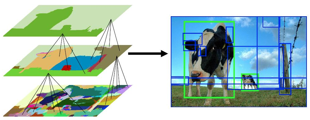
Each proposed region is then warped to a fixed size of pixels and processed independently through a pre-trained CNN (originally AlexNet) to extract a 4096-dimensional feature vector. This feature extraction step leverages the powerful representations learned by CNNs on large-scale image classification datasets, transferring this knowledge to the detection task. Finally, these CNN features are fed to class-specific Support Vector Machine (SVM) classifiers for object classification and linear regressors for bounding box refinement.
Mathematically, for a region proposal with extracted CNN features , the classification score for class is computed as:
where and are the learned SVM parameters for class . The bounding box regression predicts corrections to transform the proposal coordinates to better align with the ground truth:
While R-CNN achieved breakthrough detection performance on benchmark datasets, it suffered from significant computational inefficiencies and training complexity. Each of the 2,000 proposals required a separate forward pass through the CNN, making both training and inference extremely slow—processing a single image could take minutes. The multi-stage training process required pre-training the CNN on ImageNet, training SVMs for classification, and training linear regressors for bounding box refinement, making the pipeline complex and difficult to optimize end-to-end.
Fast R-CNN: shared computation breakthrough.
Fast R-CNN††margin: Introduced by Girshick (2015), Fast R-CNN addressed the computational bottlenecks of R-CNN while maintaining the two-stage paradigm and improving detection accuracy. addressed these limitations through a key architectural innovation: shared computation across all proposals. Instead of processing each proposal independently through the CNN, Fast R-CNN processes the entire input image once through a convolutional backbone to generate a feature map, then extracts proposal-specific features from this shared representation. This process is illustrated in the referenced figure.
The central innovation is the Region of Interest (RoI) pooling layer, which extracts fixed-size feature representations from variable-sized proposal regions on the shared feature map. For a proposal with coordinates on a feature map with spatial dimensions , RoI pooling divides the proposal region into a regular grid (typically ) and applies max pooling within each grid cell, as shown in Figure 10.2.
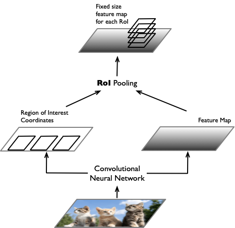
where represents the spatial extent of the -th grid cell. This operation ensures that regardless of the input proposal size, the output is always a fixed feature tensor, where is the number of feature channels.
Fast R-CNN also unified the training process through a multi-task loss function that jointly optimizes classification and bounding box regression:
where is the log loss for true class with predicted class probabilities , and is the smooth L1 loss for bounding box regression. The indicator function ensures that bounding box loss is only computed for positive examples (background class has ), and balances the two loss terms.
This architectural change provided substantial improvements in both computational efficiency and detection accuracy. By sharing CNN computation across all proposals, Fast R-CNN reduced training time by an order of magnitude while achieving higher mean Average Precision (mAP) on standard benchmarks. The end-to-end training also eliminated the complex multi-stage optimization procedure, making the system more practical for real-world deployment. However, Fast R-CNN still relied on external region proposal algorithms like selective search, which remained a computational bottleneck and prevented the entire detection pipeline from being truly end-to-end learnable. This limitation motivated the development of learnable region proposal methods, which we will explore in the next section.
10.1.2 Learnable Proposals: RPN and Faster R-CNN
While Fast R-CNN significantly improved computational efficiency through shared CNN computation, it still relies on external region proposal algorithms like selective search. These traditional methods suffered from several fundamental limitations: they were computationally expensive, requiring seconds per image; they were not learned from data and thus could not adapt to specific datasets or tasks; and they created a bottleneck that prevented the entire detection pipeline from being optimized end-to-end. The Region Proposal Network (RPN) innovation addressed these limitations by making region proposal generation a learnable component within the detection framework.
Limitations of selective search.
Selective search and similar traditional proposal methods operate using hand-crafted features and heuristics that remain fixed regardless of the detection task or dataset. These algorithms typically generate thousands of proposals per image using expensive graph-based operations, with processing times often exceeding the CNN inference itself. More critically, since these methods are not learnable, they cannot benefit from the supervision available during detection training—they cannot learn which types of regions are most likely to contain objects for a specific application domain.
Region proposal network innovation.
The Region Proposal Network (RPN) represents a paradigm shift by treating proposal generation as a learned prediction task. The RPN is essentially a fully convolutional network that slides a small network over the convolutional feature map produced by the backbone CNN. At each sliding window position, the RPN simultaneously predicts multiple region proposals using a set of reference boxes called anchors.
Anchor box design principles.
Anchors serve as reference templates that cover different scales and aspect ratios at each spatial location in the feature map. For a feature map of size , the RPN generates potential proposals, where is the number of anchor templates per location. Common anchor designs use 3 scales (e.g., , , pixels) and 3 aspect ratios (e.g., 1:1, 1:2, 2:1), resulting in anchors per location.
Mathematically, for an anchor centered at position with width and height , the RPN predicts refinements to produce a final proposal:
The exponential transformation for width and height ensures positive values and provides scale-invariant parameterization.
Objectness scoring.
Unlike traditional proposal methods that use complex heuristics, the RPN performs binary classification to determine “objectness”—whether each anchor location contains an object of any class versus background. This objectness score is simpler than full multi-class classification but captures the essential information needed for proposal generation. The RPN learns to distinguish object-like regions from background using the same convolutional features that will later be used for detailed classification.
RPN loss function.
The RPN is trained using a multi-task loss that combines objectness classification and bounding box regression:
where is the log loss for binary classification, is the smooth L1 loss for box regression, and are normalization terms, and balances the two losses. The box regression loss is only computed for positive anchors (those with ), indicated by the multiplication with .
During training, anchors are assigned positive labels if they have Intersection over Union (IoU) ¿ 0.7 with any ground truth box, or if they are the highest IoU anchor for a ground truth box. Anchors with IoU ¡ 0.3 are assigned negative labels, while those with intermediate IoU values are ignored to avoid ambiguous supervision.
Faster R-CNN: integration with Fast R-CNN.
Faster R-CNN combines the RPN with Fast R-CNN into a single, unified network that shares convolutional features between proposal generation and detection. The architecture consists of a shared CNN backbone (e.g., VGG-16 or ResNet), followed by two sibling branches: the RPN for generating proposals and the Fast R-CNN detection head for classifying proposals and refining their locations.
The shared backbone is crucial for computational efficiency—rather than running separate CNNs for proposal generation and detection, both tasks operate on the same feature representation. This sharing also enables the network to learn features that are beneficial for both tasks simultaneously.
Training strategies.
Training Faster R-CNN requires careful coordination between the RPN and detection components. Initial approaches alternated between training the RPN and the detection network. First, the RPN is trained using ImageNet-pretrained features. Then, the detection network is trained using proposals from the trained RPN, fine-tuning the shared convolutional layers. This process can be repeated, though diminishing returns are typically observed after the first iteration.
Today, most training of both components is done simultaneously, using a combined loss function:
Joint training is more efficient and often achieves better performance, as it allows the RPN and detection network to adapt to each other during learning.
Non-maximum suppression and post-processing.
After the RPN generates proposals, Non-Maximum Suppression (NMS) removes redundant detections. The algorithm sorts proposals by objectness score and iteratively removes proposals that have high IoU (typically ¿ 0.7) with higher-scored proposals. This reduces the number of proposals fed to the detection stage from thousands to hundreds, improving computational efficiency while maintaining detection quality.
The complete Faster R-CNN pipeline processes an image through the shared backbone, generates scored proposals via RPN with NMS post-processing, extracts RoI features for the top proposals, and produces final classifications and refined bounding boxes. This end-to-end learnable system achieved significant improvements in both speed and accuracy over previous two-stage methods, establishing the foundation for modern object detection architectures.
10.1.3 One-Stage Detection: YOLO
The Region Proposal Network represented a major breakthrough by making proposal generation learnable, but it still required a two-stage pipeline where proposals were generated first and then classified separately. This sequential approach, while effective, created computational bottlenecks that limited real-time performance in robotics applications. As autonomous vehicles, drones, and mobile robots demanded faster detection systems for dynamic environments, a fundamental question emerged: could object detection be reformulated to predict bounding boxes and classes directly from image features in a single forward pass?
You Only Look Once (YOLO)††margin: Introduced by Redmon et al. (2016), YOLO revolutionized object detection by demonstrating that competitive detection performance could be achieved through direct single-stage prediction, enabling real-time performance for robotics applications. provided a radical answer to this question. Rather than decomposing detection into proposal generation followed by classification, YOLO treats object detection as a single regression problem, directly predicting bounding box coordinates and class probabilities from image pixels in one evaluation of the network. This paradigm shift eliminated the computational overhead of generating and processing thousands of proposals, enabling genuine real-time object detection suitable for robotics systems operating in dynamic environments.
Core YOLO innovation: grid-based direct detection.
YOLO’s central innovation lies in its spatial decomposition of the detection problem through a grid-based approach. The method divides the input image into an grid (typically for the original YOLO), where each grid cell becomes responsible for detecting objects whose center points fall within that cell’s spatial region. This responsibility assignment creates a natural spatial organization that eliminates the need for separate proposal generation.
Each grid cell simultaneously predicts multiple bounding boxes along with their associated confidence scores and class probabilities. The key insight is that this grid-based spatial division provides sufficient spatial coverage while maintaining computational tractability—rather than evaluating thousands of potential object locations as in proposal-based methods, YOLO evaluates a fixed number of predictions per grid cell, resulting in a manageable total number of predictions regardless of scene complexity. The elimination of the proposal generation stage represents more than just a computational optimization; it fundamentally changes how the network approaches object detection. Rather than learning to generate good proposals and then classify them, the network must learn to directly map from image features to final detection outputs. This end-to-end learning enables the network to optimize the entire detection pipeline jointly, potentially leading to better coordination between localization and classification components.
YOLO architecture and predictions.
The YOLO architecture consists of a single CNN backbone followed by fully connected layers that produce the final detection tensor. The original implementation used a modified GoogLeNet architecture as the backbone, processing input images of size pixels through convolutional layers that progressively reduce spatial resolution while increasing feature depth. The final convolutional features are flattened and processed through fully connected layers to produce a structured output tensor.
The network’s output is a tensor of size , where is the grid size, is the number of bounding boxes predicted per cell, and is the number of object classes. For the original YOLO trained on PASCAL VOC, this results in a tensor, with bounding boxes and classes. Each bounding box prediction consists of five values: , where represents the box center relative to the grid cell boundaries, represents the box dimensions relative to the entire image, and confidence represents the model’s certainty that the box contains an object. The class predictions are formulated as conditional probabilities , representing the probability of each class given that an object is present in the cell. This conditional formulation is crucial—each grid cell predicts only one set of class probabilities regardless of the number of bounding boxes, reflecting the assumption that each cell is responsible for at most one object class.
The final detection confidence for each bounding box is computed by multiplying the conditional class probabilities with the bounding box confidence scores:
This formulation ensures that high detection scores require both confident object presence and accurate localization.
Loss function and training.
YOLO’s loss function addresses the multi-task nature of the detection problem by combining coordinate regression, confidence prediction, and classification into a unified objective. The loss function consists of several components with different weights to balance their relative importance:
The loss function uses different weights for different components: increases the importance of coordinate predictions, while decreases the weight of confidence predictions for cells without objects. The square root transformation for width and height helps the loss function treat errors in small and large boxes more equally, since a small absolute error in a small box represents a larger relative error than the same absolute error in a large box.
The indicator function denotes whether cell contains an object and bounding box is responsible for that prediction (determined by which predicted box has the highest IoU with the ground truth). This responsibility assignment is crucial for training stability, as it ensures each ground truth object is associated with exactly one predicted bounding box. Training YOLO follows a two-stage approach: the convolutional layers are first pre-trained on ImageNet for classification, then the entire network is fine-tuned on detection data. The classification pre-training provides the network with strong feature representations that are then adapted for the detection task. During detection training, the learning rate is carefully adjusted to balance the different loss components and ensure stable convergence.
Speed versus accuracy trade-offs and robotics impact.
YOLO’s architectural design prioritizes computational efficiency, achieving detection speeds that were unprecedented at the time of its introduction. The original YOLO processes images at 45 frames per second (FPS) on contemporary GPU hardware, while a faster variant (Fast YOLO) achieved 155 FPS by using a smaller network architecture. These speeds represent order-of-magnitude improvements over contemporary two-stage methods like Fast R-CNN, which operated at approximately 7 FPS. However, this speed comes with accuracy trade-offs. YOLO’s grid-based approach struggles with small objects, since multiple small objects within the same grid cell cannot be detected independently. The method also has difficulty with objects that appear in unusual aspect ratios, as the fixed number of bounding box predictors per cell limits the diversity of detectable shapes. Additionally, the coarse spatial quantization imposed by the grid structure can lead to less precise localization compared to methods that can place proposals at arbitrary locations.
For robotics applications, these trade-offs often represent acceptable compromises. Autonomous vehicles operating in real-time require detection systems that can process sensor data fast enough to support control decisions, even if absolute detection accuracy is somewhat reduced. The “good enough” detection philosophy embodied by YOLO aligns well with robotics applications where timely decisions often matter more than perfect perception. The impact of YOLO on the robotics field extends beyond its specific technical contributions. By demonstrating that real-time object detection was achievable with modest computational resources, YOLO democratized object detection for resource-constrained robotics platforms. Mobile robots, drones, and embedded systems could now incorporate sophisticated visual understanding capabilities without requiring expensive computational hardware.
The evolution of YOLO through subsequent versions (YOLOv2, YOLOv3, YOLOv4, YOLOv5, and beyond) has addressed many of the original accuracy limitations while maintaining the core computational advantages. Modern YOLO variants incorporate multi-scale feature processing, improved loss functions, and architectural refinements that close much of the accuracy gap with two-stage methods while preserving real-time performance. This progression demonstrates the enduring value of the single-stage detection paradigm for robotics applications where speed and efficiency are paramount.
10.1.4 Transformer-Based Object Detection
Transformers have recently been adapted to tackle object detection, and their performance shows several benefits over CNN-based models. Detection Transformers (DETR)11. Carion, Nicolas, Massa, Francisco, Synnaeve, Gabriel, Usunier, Nicolas, Kirillov, Alexander, Zagoruyko, Sergey. “End-to-End Object Detection with Transformers.” In Computer Vision – ECCV 2020, 213–229. Springer International Publishing, 2020., illustrated in Figure 10.3, propose to formulate the object detection problem as a direct set prediction problem, largely streamlining the detection pipeline through its end-to-end structure. In its most basic form, DETR is an end-to-end Transformer model that takes in images as inputs and predicts a fixed set of potential bounding boxes. DETR removes many hand-designed components, including “region proposal” and “non-maximum suppression” that are commonly used in CNN-based models.

Specifically, DETR uses a conventional CNN backbone to learn 2D feature maps from an input image, as shown on the left side of Figure 10.4. The model then converts the 2D feature maps into a sequence of feature tokens, similarly to Vision Transformers. These tokenized features are further fed into a Transformer encoder, comprised of a stack of self-attention mechanisms and multi-layer perceptrons, for further feature encoding. The encoded sequence is processed by a Transformer decoder that relates the feature sequence with a set of “learnable object queries”. These object queries encode the distribution of object information, including size, location, and category, over an image.
Note that Transformer decoders have some key differences from encoders. For example, they can use what we refer to as cross-attention layers and masked attention layers. We use cross-attention layers to allow a sequence to get contextual information from another sequence, unlike self-attention layers which gather contextual information from within a single sequence. In the context of DETR, this allows the decoder to relate the encoder’s feature embeddings to the object queries, which are two different input sets.
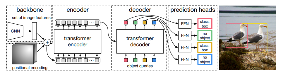
Finally, each object query, after absorbing image features, is processed by shared fully connected layers to predict class labels, bounding box centers, and bounding box sizes. A “no object” label is assigned to queries without true objects detected, allowing the model to handle a variable number of objects in an image. In contrast to CNN-based object detectors, Transformer-based object detectors do not have one-to-one matching between the prediction set and the ground-truth set. Therefore, a set-based loss is used to produce an optimal bipartite matching between predicted and ground-truth objects, followed by optimizing object-centric (bounding box) losses.
10.2 3D Object Detection
While 2D object detection provides valuable information about what objects are present and their approximate locations in images, many robotics applications require understanding the full 3D structure and pose of objects in the physical world. Consider a robotic arm performing pick-and-place operations—knowing that a cup appears in a specific region of an image is insufficient for grasping; the robot needs the cup’s precise 3D location, orientation, and dimensions to plan a successful grasp trajectory. Similarly, autonomous vehicles must understand the 3D positions and velocities of surrounding cars, pedestrians, and obstacles to make safe navigation decisions in real-world coordinates rather than image pixels. The transition from 2D to 3D detection introduces changes in problem formulation, data representation, and evaluation metrics while preserving many of the core architectural principles developed for 2D detection. Understanding these extensions provides the foundation for building robust 3D detection systems using the point cloud and voxel processing architectures from the previous chapter.
10.2.1 Extending Object Detection to 3D
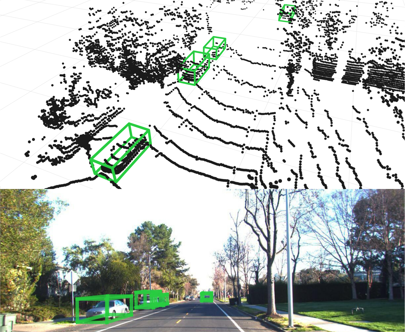
3D object detection extends the 2D formulation by instead predicting 3D bounding boxes to represent objects in three-dimensional space. While 2D detection outputs bounding boxes parameterized by in image coordinates, 3D detection requires additional parameters to specify the object’s full pose and extent. Examples of 3D object detection in autonomous driving scenarios are shown in Figure 10.5.
Definition 10.1 (3D object detection).
Given 3D sensor data (point cloud, voxel grid, or RGB-D), 3D object detection aims to identify all instances of objects from a predefined set of classes and localize each instance with a 3D bounding box. The output is a set of 3D detections where represents the 3D bounding box with center coordinates , dimensions for length, width, and height, and orientation .
Extending anchor design to 3D space.
For 3D anchor design, each anchor is parameterized by seven values: representing the center coordinates, dimensions, and orientation. Common 3D anchor designs use aspect ratios appropriate for the target object classes, and discrete orientation bins (e.g., 0°, 90°, 180°) to handle rotation invariance.
The anchor refinement process follows similar principles to 2D detection, with the network predicting corrections to transform anchor parameters into final detections:
Similar to 2D setting, the exponential transformation ensures positive dimensions, while orientation is handled through additive corrections with appropriate normalization to handle angle wraparound.
Two-stage versus one-stage paradigms in 3D.
The two-stage and one-stage detection paradigms from 2D systems transfer directly to 3D detection, with each approach offering distinct advantages for different 3D data modalities and applications. Two-stage 3D detectors follow the proposal-then-classification paradigm, first generating 3D object proposals from point clouds or voxel grids, then refining these proposals through dedicated classification and regression heads. This approach works particularly well with point-based representations, where the first stage can identify promising object centers using techniques like Hough voting, and the second stage can perform detailed classification using local point features. One-stage 3D detectors perform classification and localization simultaneously, making them better suited for real-time robotics applications where latency is critical. These methods work well with regular voxel or pillar representations that enable efficient convolutional processing across the entire 3D space. The choice between paradigms often depends on the input data modality: point-based methods naturally lend themselves to two-stage approaches due to the irregular nature of point clouds, while voxel-based methods can efficiently implement one-stage detection using 3D CNNs.
Non-maximum suppression in 3D.
Non-Maximum Suppression extends to 3D by replacing 2D IoU calculations with 3D IoU or Bird’s Eye View (BEV) IoU metrics. 3D IoU computes the overlap between two 3D bounding boxes in full 3D space, accounting for differences in position, size, and orientation:
Computing 3D IoU requires determining the intersection volume between two oriented 3D boxes, which is more complex than the 2D case but essential for accurate duplicate removal.
For autonomous driving applications, BEV IoU is often preferred as it focuses on the ground plane where most objects interact:
where represents the projection of the 3D bounding box onto the ground plane. BEV IoU is computationally simpler and often more relevant for navigation tasks.
Evaluation metrics for 3D detection.
3D object detection uses specialized metrics that account for spatial dimensions and orientation accuracy. The standard metric is 3D Average Precision (AP) computed using 3D IoU thresholds (typically 0.5 and 0.7). For autonomous driving, evaluation often focuses on Bird’s Eye View (BEV) metrics that emphasize horizontal plane accuracy, with benchmarks like KITTI providing difficulty-based analysis. Orientation accuracy is measured through angular error between predicted and ground truth orientations, with some metrics requiring joint spatial and angular tolerance for correct detections.
10.2.2 3D Detection from Point Clouds and Voxel Representations
Building effective 3D object detection systems requires leveraging the specialized architectures for 3D data processing developed in the previous chapter. The choice between point-based and voxel-based representations fundamentally shapes the detection architecture, with each approach offering distinct advantages for different robotics applications. Point-based methods preserve the geometric precision of the original sensor data and handle irregular point distributions naturally, making them well-suited for applications requiring precise object localization. Voxel-based methods trade some geometric precision for computational efficiency by imposing regular grid structures that enable optimized convolutional operations, making them preferred for real-time robotics applications.
Rather than being mutually exclusive, these representations often complement each other within detection pipelines. Many successful 3D detection systems combine the efficiency of voxel processing for initial feature extraction with the precision of point-based refinement for final object localization. Understanding how different detection paradigms—two-stage, one-stage, and transformer-based—can be adapted to work with these 3D representations provides the foundation for building robust detection systems.
Leveraging 3D feature representations.
The 3D detection architectures we will explore build directly upon the feature extraction capabilities of PointNet, VoxelNet, and PointPillars discussed in the previous chapter. These architectures provide learned feature representations that encode geometric patterns, spatial relationships, and semantic information from 3D sensor data. The key insight is that these features can serve as input to detection heads that predict object classifications and 3D bounding box parameters.
Point-based representations excel at preserving fine-grained geometric details and handling the irregular structure of sensor data. PointNet++ features capture multi-scale geometric patterns through hierarchical set abstraction, enabling detection of objects at different scales and levels of detail. These features are particularly valuable for detecting small objects or distinguishing between closely spaced instances where geometric precision is critical. Voxel-based representations provide computational advantages through regular grid structures that enable efficient 3D convolutions and parallel processing. VoxelNet features encode local geometric patterns within voxels while maintaining spatial relationships across the scene. PointPillars features offer a hybrid approach, encoding vertical structure within pillars while enabling efficient 2D processing for large-scale scenes. The choice between these representations often depends on the computational constraints and accuracy requirements of the specific robotics application.
10.2.3 Two-Stage 3D Detection: Extending Faster R-CNN
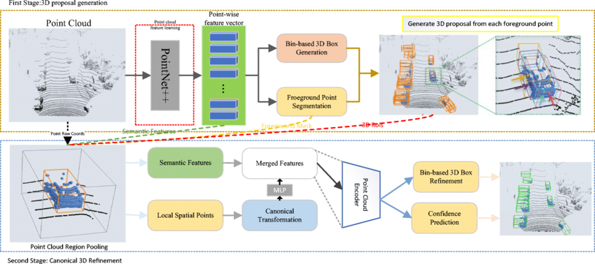
The two-stage detection paradigm extends naturally to 3D by first generating object proposals in 3D space, then refining these proposals through dedicated classification and regression networks. This approach works particularly well when combined with the hierarchical feature representations from PointNet++ or the structured features from VoxelNet. The PointRCNN architecture is illustrated in Figure 10.6.
PointRCNN: point-based two-stage detection.
PointRCNN demonstrates how the Faster R-CNN paradigm can be adapted to work directly with point cloud data using PointNet++ features. The architecture follows a bottom-up approach where object proposals are generated directly from point-wise features rather than through dense sliding window approaches used in image detection.
The first stage leverages PointNet++ hierarchical features to perform point-wise binary classification, identifying points that likely belong to foreground objects versus background. Rather than generating proposals at regular grid locations, PointRCNN generates 3D proposals centered at high-confidence foreground points. This approach is computationally efficient because it only considers a subset of points for proposal generation, and it preserves the geometric precision of the original point cloud. For each proposal, the second stage extracts local point features within the proposed 3D region and applies canonical coordinate transformation to normalize the local geometry. This transformation aligns the object coordinate system with a canonical orientation, making the subsequent classification and regression tasks more robust to object orientation variations. The canonical transformation is particularly important for 3D detection because objects can appear in arbitrary orientations in the sensor coordinate system.
The mathematical formulation for the canonical transformation involves rotating and translating the local point coordinates so that the object’s principal axes align with canonical directions:
where is the estimated object rotation and is the estimated object center. This transformation enables the network to learn object-centric features that are invariant to the object’s pose in the world coordinate system.
VoxelNet: voxel-based two-stage detection.
VoxelNet adapts the two-stage paradigm to work with voxel-based representations by integrating Voxel Feature Encoding with Region Proposal Network concepts. The architecture processes point clouds through VFE layers to generate voxel-wise features, then applies 3D convolutional layers to build hierarchical representations across the voxelized space. The proposal generation stage adapts the RPN concept to 3D by sliding 3D anchor templates across the feature volume. At each spatial location in the 3D feature map, the network predicts objectness scores and 3D bounding box refinements for multiple anchor templates covering different object sizes and orientations. The 3D RPN loss combines objectness classification with 3D bounding box regression:
where incorporates losses for all seven parameters of the 3D bounding box: center coordinates, dimensions, and orientation.
The second stage performs 3D RoI pooling to extract fixed-size features for each proposal, followed by classification and bounding box refinement. The 3D RoI pooling operation extends the 2D concept by pooling features from 3D regions of the feature volume, maintaining spatial relationships in all three dimensions.
10.2.4 One-Stage 3D Detection: Direct Prediction
One-stage 3D detection methods perform object classification and localization simultaneously, eliminating the separate proposal generation stage. These approaches are particularly well-suited for real-time robotics applications where detection latency must be minimized.
CenterPoint: treating 3D objects as points.
CenterPoint represents objects as points in Bird’s Eye View (BEV) space and performs detection through keypoint estimation, similar to 2D anchor-free methods like CenterNet. The approach builds on PointPillars pillar-based representation to efficiently process large-scale point clouds while maintaining real-time performance.
The key insight is that 3D objects can be effectively represented by their center points when projected into BEV space, particularly for autonomous driving scenarios where objects primarily move on the ground plane. CenterPoint predicts a heatmap in BEV coordinates where peaks correspond to object centers, along with regression maps that predict 3D bounding box parameters for each detected center. The detection pipeline processes point clouds through PointPillars to generate BEV feature maps, then applies 2D convolutional networks to predict center heatmaps and regression targets:
where represents the BEV feature map from PointPillars processing, and is the sigmoid activation for heatmap prediction. The regression targets include 3D center offsets, object dimensions, and orientation angles.
The loss function combines center point detection with regression objectives:
where uses focal loss to handle the extreme imbalance between center points and background, and uses smooth L1 loss for the continuous regression targets. CenterPoint extends beyond basic detection by incorporating velocity estimation for tracking applications. By processing consecutive frames, the network can predict object velocities directly as part of the regression targets, enabling seamless integration with multi-object tracking systems essential for autonomous navigation.
10.2.5 Transformer-Based 3D Detection
Transformer architectures have been successfully adapted to 3D detection by treating object detection as a set prediction problem, eliminating the need for hand-designed anchors and complex post-processing steps like non-maximum suppression.
3DETR: set-to-set prediction in 3D.
3DETR extends the DETR paradigm to 3D object detection by using transformer architectures to directly predict sets of 3D bounding boxes from point cloud or voxel features. The approach uses learnable object queries that attend to 3D scene features through cross-attention mechanisms, enabling end-to-end learning from raw 3D data to final detections. The architecture processes 3D input data through feature extraction networks (PointNet++ for point clouds or 3D CNNs for voxel grids) to generate scene feature representations. These features are then processed by a transformer encoder to build contextual representations that capture long-range dependencies across the 3D scene. The transformer decoder uses a fixed set of learnable object queries to attend to the encoded scene features and predict object detections.
Each object query learns to specialize in detecting objects with particular characteristics or in specific spatial regions. The cross-attention mechanism allows queries to gather relevant information from across the entire scene, enabling detection of partially occluded objects or objects that extend across multiple local regions. The self-attention within the decoder enables queries to coordinate with each other, reducing duplicate detections without explicit post-processing. The final prediction heads convert each object query’s representation into 3D bounding box parameters and class predictions:
where is the -th object query after transformer processing. The training uses Hungarian matching to establish optimal assignment between predicted and ground truth objects, followed by standard detection losses.
The set-based prediction eliminates the need for anchor design, anchor assignment strategies, and non-maximum suppression, simplifying the detection pipeline while achieving competitive performance. This approach is particularly attractive for complex 3D scenes where traditional anchor-based methods struggle with the high-dimensional anchor space and complex object interactions.
10.3 Semantic and Instance Segmentation
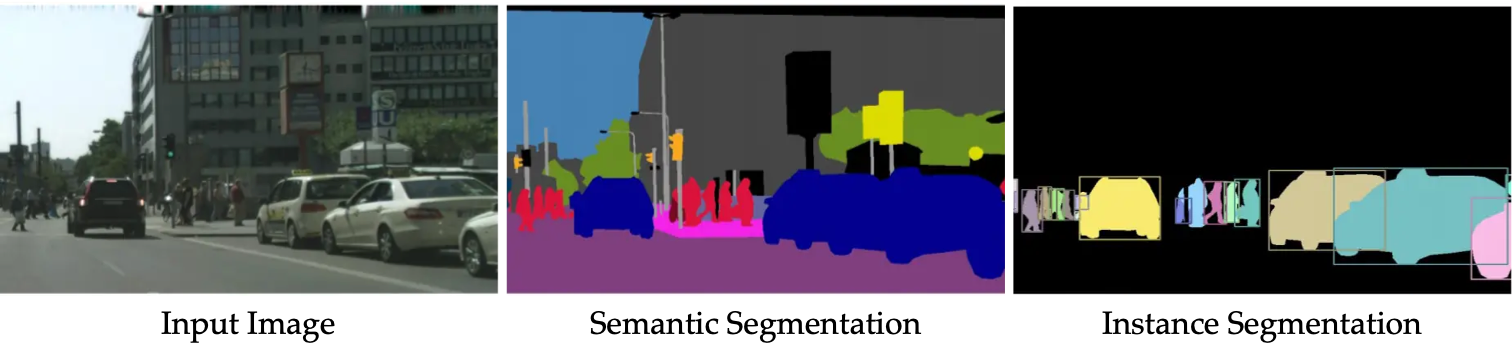
Segmentation extends object detection by providing pixel-level or point-level understanding of scenes, enabling robots to understand not just where objects are located, but precisely which pixels belong to each object or scene category. While object detection provides coarse spatial understanding through bounding boxes, segmentation offers fine-grained spatial reasoning essential for tasks like autonomous navigation on complex terrain, precise robotic manipulation, and detailed scene understanding. Figure 10.7 illustrates an example of semantic and instance segmentation outputs.
10.3.1 Semantic Segmentation
Semantic segmentation extends image understanding beyond object detection by classifying every pixel in an image into predefined semantic categories, providing dense spatial understanding of the scene. Unlike object detection which outputs sparse bounding boxes, semantic segmentation produces pixel-level predictions that preserve the precise boundaries and spatial extent of different scene elements. This fine-grained understanding is essential for robotics applications where precise spatial reasoning is required.
Problem definition and robotics applications.
Semantic segmentation performs pixel-level classification without distinguishing between different instances of the same class. For an input image of size , the output is a segmentation map of the same spatial dimensions, where each pixel is assigned a class label from the predefined set of semantic categories. For robotics systems, autonomous vehicles use segmentation to identify drivable road surfaces, distinguish between different types of terrain, and understand scene layout for path planning. Mobile robots navigating indoor environments use segmentation to identify floors, walls, furniture, and obstacles, enabling more sophisticated spatial reasoning for navigation planning. In each case, the pixel-level precision enables robots to make more informed decisions about how to interact with their environment.
Fully convolutional networks (FCNs).
Semantic segmentation can be viewed as dense classification where standard CNN architectures are adapted to produce spatial output maps rather than single classification scores. Fully Convolutional Networks (FCNs) build on the convolutional feature extraction capabilities of CNNs while replacing the fully connected classification layers with convolutional layers that preserve spatial structure. These models replace the fully connected layers typically used for classification with convolutional layers that can accept images of arbitrary size and produce correspondingly sized output maps. For a CNN backbone that produces feature maps of size (due to pooling operations), FCN applies convolutions to produce class score maps, then upsamples these maps back to the original image resolution. The upsampling process uses transposed convolutions (also called deconvolutions) to increase spatial resolution:
where is the upsampling stride and represents the learned transposed convolution weights. This operation is the mathematical inverse of convolution with stride , enabling learnable upsampling that can recover spatial details.
FCN introduces skip connections that combine features from different layers of the encoder to recover fine-grained spatial information lost during downsampling. These connections add feature maps from earlier layers (with higher spatial resolution) to upsampled feature maps from deeper layers (with richer semantic information):
This fusion enables the network to combine high-level semantic understanding with low-level spatial precision, crucial for accurate boundary delineation in robotics applications.
U-Net and encoder-decoder architectures.
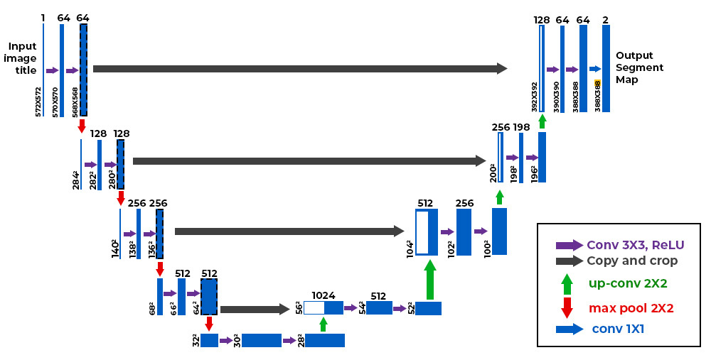
U-Net represents a systematic approach to encoder-decoder architectures that has become foundational for semantic segmentation across many domains. The U-Net architecture, illustrated in Figure 10.8, consists of a contracting path (encoder) that progressively reduces spatial resolution while increasing feature depth, followed by an expansive path (decoder) that gradually recovers spatial resolution while combining features across scales. For each decoder layer, skip connections concatenate features from corresponding encoder layer:
where denotes concatenation and UpConv represents upsampling convolution operations. These skip connections preserve fine-grained spatial details that would otherwise be lost during the encoding process.
The symmetric design ensures that the decoder has access to features at multiple scales, enabling accurate segmentation of both large objects (captured by deep, low-resolution features) and fine details (preserved through skip connections from high-resolution features). This multi-scale feature combination is particularly important for robotics applications where accurate boundary detection affects safety and task performance.
Training loss: classification cross-entropy per pixel.
Semantic segmentation networks are trained using pixel-wise classification loss, treating each pixel as an independent classification problem. The standard loss function is cross-entropy computed across all pixels:
where is the ground truth one-hot encoding for pixel and class , and is the predicted probability. This formulation treats each pixel independently, enabling efficient batch processing and straightforward optimization.
However, pixel-wise cross-entropy can struggle with class imbalance, which is common in robotics scenarios where background pixels often dominate the scene. Various modifications address this challenge, including weighted cross-entropy that assigns different weights to different classes based on their frequency, and focal loss that emphasizes hard examples by down-weighting well-classified pixels.
10.3.2 Instance Segmentation
Instance segmentation combines object detection and semantic segmentation by identifying individual object instances and their precise pixel-level boundaries. Unlike semantic segmentation which treats all objects of the same class identically, instance segmentation distinguishes between separate instances—for example, identifying three individual cars rather than just “car pixels”. This capability is critical for robotics applications where understanding individual objects enables targeted interaction and manipulation.
Problem definition and distinction from semantic segmentation.
Instance segmentation extends semantic segmentation by assigning unique instance identifiers to pixels belonging to distinct objects. For an input image, the output includes both semantic labels and instance masks, where each instance mask defines the pixel-level extent of the -th detected object instance. The key distinction is that semantic segmentation answers “what is this pixel?” while instance segmentation answers “what is this pixel and which specific object does it belong to?” For a robotic arm grasping objects from a bin, semantic segmentation might identify all pixels as “tool,” but instance segmentation identifies individual wrenches, screwdrivers, and hammers, enabling the robot to select and grasp specific items.
Mask R-CNN: extending detection with segmentation.
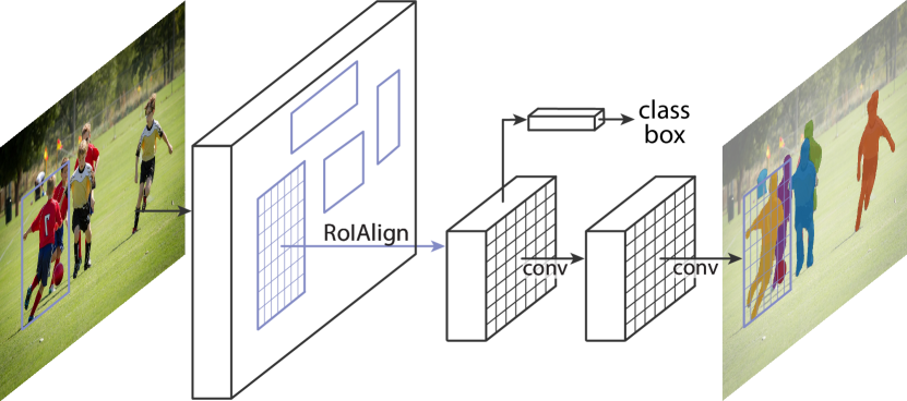
Mask R-CNN, illustrated in Figure 10.9, extends Faster R-CNN by adding a segmentation branch that predicts pixel-level masks for each detected object. The architecture maintains the two-stage paradigm: the RPN generates object proposals, and the detection head performs classification, bounding box regression, and mask prediction. The key innovation is RoI Align, which replaces RoI pooling to address spatial misalignment issues. While RoI pooling quantizes proposal coordinates to discrete feature map positions, RoI Align uses bilinear interpolation to sample features at exact locations:
This precise alignment is essential for accurate mask prediction, as small spatial misalignments can significantly degrade segmentation quality.
The mask prediction branch applies a small FCN to each RoI-aligned feature to produce a binary mask for the predicted object class. The mask loss is computed only for the predicted class to avoid competition between classes:
where is the predicted class, is the ground truth mask, and is the predicted mask for class .
Panoptic segmentation.
Panoptic segmentation unifies semantic and instance segmentation by providing complete scene understanding. The task divides semantic categories into ”things” (countable objects like cars, people) and ”stuff” (amorphous regions like sky, road), performing instance segmentation for things and semantic segmentation for stuff. For robotics applications, panoptic segmentation provides comprehensive scene understanding. An autonomous vehicle can simultaneously understand the road surface (stuff), individual vehicles and pedestrians (thing instances), and background elements like buildings and vegetation (stuff), enabling holistic reasoning about the driving environment.
Bottom-up approaches.
Bottom-up instance segmentation methods first perform pixel-level feature learning, then group pixels into instances based on learned embeddings. These approaches contrast with top-down methods like Mask R-CNN that first detect objects then segment them. Associative embedding learns pixel-level features where pixels belonging to the same instance have similar embedding vectors, while pixels from different instances have dissimilar embeddings. Instance masks are then generated by clustering pixels in the embedding space:
where and are embedding vectors for pixels and . Pixels with distances below a threshold are grouped into the same instance.
These methods can handle arbitrary numbers of instances without predefined proposals but require robust clustering algorithms to separate instances reliably. They are particularly useful for robotics scenarios with dense object arrangements where proposal-based methods might struggle.
10.3.3 3D Segmentation
3D segmentation extends pixel-level understanding to volumetric data, providing precise spatial reasoning for robotics applications that require detailed 3D scene understanding. While 2D segmentation enables robots to understand image content, 3D segmentation allows reasoning about the full spatial extent and structure of objects in the physical world. This capability is essential for manipulation tasks requiring grasp planning, navigation in complex 3D environments, and understanding object affordances based on geometric structure.
Point cloud segmentation.
Point cloud segmentation assigns semantic labels or instance identifiers to individual points in 3D space. The formulation extends 2D segmentation concepts to irregular point data, where each point receives a label for semantic segmentation or instance identifier for instance segmentation. Semantic segmentation of point clouds using PointNet++ leverages the hierarchical set abstraction layers from the previous chapter. The architecture processes points through multiple scales of local feature extraction and aggregation, then applies classification heads to predict semantic labels for each point:
where represents the final point-wise feature after layers of hierarchical processing. The multi-scale feature extraction enables accurate segmentation of objects at different sizes and levels of detail.
Instance segmentation in point clouds requires additional mechanisms to group points into distinct object instances. Methods like PointGroup combine semantic segmentation with learned offset vectors that point toward instance centers, enabling clustering of points belonging to the same object. The training loss combines semantic classification with offset regression:
where encourages points to predict vectors pointing toward their instance centers, and promotes tight clustering within instances and separation between instances.
Voxel-based segmentation.
Voxel-based segmentation processes regular 3D grids where each voxel represents a volumetric unit in 3D space. The formulation treats segmentation as 3D dense classification, where each voxel receives a semantic label or occupancy prediction. Occupancy grids represent a fundamental approach where each voxel indicates whether that region of space is occupied by an object. This binary classification provides essential information for navigation and collision avoidance:
where represents the occupancy probability for voxel .
3D U-Net architectures extend the encoder-decoder paradigm to volumetric data for detailed semantic segmentation. The architecture applies 3D convolutions throughout the encoding and decoding paths, with 3D skip connections preserving spatial details:
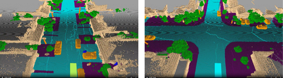
The 3D convolutions capture volumetric patterns and spatial relationships essential for accurate 3D segmentation, while skip connections ensure fine-grained geometric details are preserved in the final predictions. An example of 3D voxel-based segmentation is shown in Figure 10.10.
10.3.4 Robotics-Specific Applications
Segmentation enables several critical robotics capabilities that require detailed geometric understanding of objects and environments. We explore a few examples below.
Example 10.3.1.
Grasp point prediction through part segmentation identifies functional regions of objects that are suitable for robotic grasping. By segmenting objects into semantic parts (handles, graspable surfaces, fragile regions), robots can plan grasps that are both mechanically sound and functionally appropriate. For example, segmenting a mug into handle, rim, and body regions enables the robot to choose appropriate grasp locations based on the intended manipulation task.
Example 10.3.2.
Terrain traversability analysis uses 3D segmentation to classify different terrain types and their suitability for robot navigation. Outdoor mobile robots use segmentation to distinguish between solid ground, obstacles, vegetation, and hazardous terrain, enabling safe path planning in complex outdoor environments. The 3D understanding allows reasoning about terrain slope, roughness, and stability that would be impossible with 2D analysis alone.
Example 10.3.3.
Object affordance understanding through part-based analysis enables robots to reason about how objects can be used based on their geometric structure. By segmenting objects into functional parts and understanding the spatial relationships between parts, robots can infer possible interactions and manipulation strategies. A segmented chair with identified seat, backrest, and legs enables the robot to understand both the object’s function and how to manipulate it safely.
These applications demonstrate how 3D segmentation provides the detailed spatial understanding necessary for robots to interact effectively with complex 3D environments, going beyond simple object detection to enable sophisticated reasoning about object structure, function, and manipulation possibilities.
10.4 Summary
In this chapter, we explored the essential robotic perception tasks of object detection and segmentation, which provide the spatial understanding necessary for robots to interact intelligently with their environments.
We began with the foundations of 2D object detection, contrasting the two-stage paradigm—exemplified by the evolution from R-CNN to the efficient, learnable proposals of Faster R-CNN—with the one-stage paradigm of YOLO, which prioritizes speed for real-time applications. We also discussed how the Transformer architecture has been adapted for detection with models like DETR, which simplify the pipeline by framing detection as a direct set prediction problem. We then extended these concepts to 3D, detailing how detection paradigms adapt to point cloud and voxel data. We covered two-stage point-based methods like PointRCNN, one-stage voxel-based methods like CenterPoint, and Transformer-based approaches like 3DETR, each offering different trade-offs between precision and computational efficiency for processing 3D sensor data.
Finally, we delved into segmentation, which provides pixel- and point-level understanding. We covered semantic segmentation with architectures like FCN and U-Net for categorizing every pixel, instance segmentation with Mask R-CNN for identifying individual objects, and their unification in panoptic segmentation. We further extended these ideas to 3D point cloud and voxel-based segmentation, highlighting their critical role in applications requiring detailed geometric reasoning, such as grasp point prediction and terrain analysis.
To learn more.
For a deeper exploration of the topics covered in this chapter, several key resources are available. The seminal papers on two-stage detection 22. Girshick, Ross. “Fast R-CNN.” In 2015 IEEE International Conference on Computer Vision (ICCV), 1440-1448, 2015. and one-stage detection 33. Redmon, J., Divvala, S., Girshick, R., Farhadi, A. “You Only Look Once: Unified, Real-Time Object Detection.” In Proceedings of the IEEE Conference on Computer Vision and Pattern Recognition (CVPR), 2016. are foundational to the field. For Transformer-based detection, the DETR paper 44. Carion, Nicolas, Massa, Francisco, Synnaeve, Gabriel, Usunier, Nicolas, Kirillov, Alexander, Zagoruyko, Sergey. “End-to-End Object Detection with Transformers.” In Computer Vision – ECCV 2020, 213–229. Springer International Publishing, 2020. introduced the set prediction paradigm. In 3D perception, the original papers on PointRCNN 55. Shi, Shaoshuai, Wang, Xiaogang, Li, Hongsheng. “PointRCNN: 3D Object Proposal Generation and Detection From Point Cloud.” In The IEEE Conference on Computer Vision and Pattern Recognition (CVPR), 2019. and VoxelNet 66. Zhou, Yin, Tuzel, Oncel. “Voxelnet: End-to-end learning for point cloud based 3d object detection.” In Proceedings of the IEEE conference on computer vision and pattern recognition, 4490–4499, 2018. are essential reading for point-based and voxel-based detection, respectively. For segmentation, the works on Mask R-CNN 77. He, Kaiming, Gkioxari, Georgia, Dollár, Piotr, Girshick, Ross. “Mask R-CNN.” In Proceedings of the IEEE International Conference on Computer Vision, 2961–2969, 2017. and U-Net 88. Olaf Ronneberger, Philipp Fischer, Thomas Brox. “U-Net: Convolutional Networks for Biomedical Image Segmentation.” CoRR abs/1505.04597, 2015. provide the basis for modern instance and semantic segmentation techniques.
10.5 Exercises
The starter code for the exercises provided below is available online through GitHub. To get started, download the code by running in a terminal window:
We denote Problems requiring hand-written solutions and coding in Python with ![[Uncaptioned image]](/book-assets/object-detection/figs__write.png) and
and ![[Uncaptioned image]](/book-assets/object-detection/figs__code.png) , respectively.
, respectively.
Problem 1: Object Detection Using Pre-trained Models
In this exercise, you will get to experiment with pre-trained computer vision models for image object detection.
Using the provided notebook
ch10/exercises/object_detection.ipynb:
-
1.
Implement the code to load and evaluate a pre-trained model for object detection.
-
2.
Implement the function draw_result to create an image with the bounding boxes, labels, and scores overlaid.
-
3.
Implement the function filter to filter the boxes, labels, and scores based on a score threshold.
Practice · 1 notebooks
- Object Detection Open in Colab Source