Finite State Machines · Principles of Robot Autonomy

The preceding parts of this book have endowed the robot with a comprehensive set of foundational competencies. In Part I, we explored how optimal control provides a powerful framework for generating and executing robot motion. Part II introduced the perceptual capabilities of the robot, examining the sensors and algorithms required to observe and interpret its environment. Part III endowed the robot with a representation of its own state within the world, covering the methods by which it estimates its pose and constructs maps of its surroundings.

In this chapter, and Part IV as a whole, we move to a higher level of abstraction: robot decision-making. Here, the focus of decision-making shifts from the fine-grained details of physical motion to the strategic choices a robot must make to achieve its long-term goals. To illustrate this distinction, consider a mission in which a robot must navigate from an initial location A to a pickup location B, retrieve a package, and deliver it to a destination C. Executing the motion from A to B relies on the planning and control techniques developed in Part I. Detecting and identifying the package requires the perceptual models of Part II, while successful navigation depends on the localization and mapping methods introduced in Part III. However, coordinating these capabilities—deciding to navigate first, then grasp the object, then proceed to the delivery location, and to monitor and recover from failures along the way—requires an additional layer of decision-making. This layer operates over a discrete set of task modes and action choices, complementing the robot’s continuous physical state.

In this chapter, we introduce finite state machines as a foundational framework for modeling and implementing discrete decision-making in robots⁷7. Kaelbling, L., White, J., Abelson, H., Freeman, D., Lozano-Pérez, T., Chuang, I. 6.01SC: Introduction to Electrical Engineering and Computer Science I. MIT OpenCourseWare, 2011.. We begin by providing a mathematical definition of a finite state machine in Section 16.1, and then discuss some architecture options, computational challenges, and practical implementation approaches in Section 16.2. Finally, in Section 16.3, we discuss the main limitations of finite state machines that motivate more advanced decision-making frameworks, which we explore in Chapters the referenced item-the referenced item.

16.1 A Mathematical Model of Discrete Decision-Making

Finite state machines (FSMs) are a computational modeling framework for systems that can be in one of a finite number of discrete states at any given time. This framework is used in a wide variety of disciplines, including electrical engineering, linguistics, computer science, philosophy, biology, and more. We can use FSMs in several different ways, including to specify a desired program or behavior, to model and analyze a system’s behavior, or to predict future behavior.

Formally, we define a FSM by a finite set of states $S$ , an input alphabet $I$ , an output alphabet $O$ , a next–state function $n:S\times I\to S$ , and an initial state $s_{0}\in S$ . Additionally, we can define an output function according to two standard conventions:

•

Mealy machine: the output depends on the current state and the current input:

$o:S\times I\to O,\qquad o_{t}=o(s_{t},i_{t}).$
•

Moore machine: the output depends only on the current state:

$\tilde{o}:S\to O,\qquad o_{t}=\tilde{o}(s_{t}).$

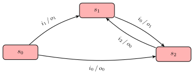
Graphically, we represent states $S$ as nodes and admissible transitions as directed edges. For a Mealy machine, each edge is typically labeled with an input/output pair $i/o$ , indicating that when input $i$ is received in state $s$ , the machine moves along that edge to $s^{\prime}=n(s,i)$ and produces output $o\!=\!o(s,i)$ . Equivalently, the output associated with a Mealy machine can be viewed as an annotation on each state–input pair $(s,i)$ . For a Moore machine, edges are labeled only by inputs^†^†margin: Since outputs do not depend on inputs. and each node is annotated with its output value.

In what follows, we adopt the Mealy convention. Unless stated otherwise, we assume a deterministic^†^†margin: In a deterministic FSM, each state has only one transition for each possible input. FSM with initial state $s_{0}$ , discrete time index $t=0,1,2,\dots$ , next state $s_{t+1}=n(s_{t},i_{t})$ , and output $o_{t}=o(s_{t},i_{t})$ . This matches the graphical convention in Figure 16.1, where nodes are states, directed edges encode input-driven transitions, and edge labels include both the triggering input and the resulting output.

diagram — Figure 16.1: A graphical representation of a FSM with states $S=\{s_{0},s_{1},s_{2}\}$ , inputs $I=\{i_{0},i_{1},i_{2}\}$ and outputs $O=\{o_{0},o_{1}\}$ . The directed edges correspond to the next-state functions and the output associated with each edge is defined by the output function. For example, in this FSM, we show the transition $n(s_{0},i_{1})\xrightarrow{}s_{1}$ in the top left, along with the corresponding output $o(s_{0},i_{1})\xrightarrow{}o_{1}$ .

Example 16.1.1 (Parking Gate Control).

Consider a parking gate control problem where the goal is to raise the gate when a car arrives, and then lower the gate when the car has passed. We assume sensors (or software events) indicate when a car is detected/cleared at the gate and when the gate reaches its end stops. The control actions are raising, lowering, or holding the gate position fixed. Note that in the real world, the position and velocity of the gate can vary continuously between the down and up positions. However, we use a higher-level discrete abstraction for the overall logic.

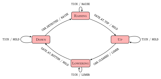
We model the FSM in Mealy style with states:

S\coloneqq\{\textsc{Down},\textsc{Raising},\textsc{Up},\textsc{Lowering}\},

an input alphabet:

I\coloneqq\{\texttt{CAR\_DETECTED},\ \texttt{CAR\_CLEARED},\ \texttt{GATE\_AT% \_TOP},\ \texttt{GATE\_AT\_BOTTOM},\ \texttt{TICK}\},

and outputs:

O\coloneqq\{\texttt{RAISE},\ \texttt{LOWER},\ \texttt{HOLD}\}.

Here TICK is a periodic control-cycle event that lets the machine command continuous motion between end-stop events.

We define the next-state and output maps $n(s,i)$ and $o(s,i)$ with representative rules:

		$\displaystyle n(\textsc{Down},\texttt{CAR\_DETECTED})=\textsc{Raising},\quad$		$\displaystyle o(\textsc{Down},\texttt{CAR\_DETECTED})=\texttt{RAISE},$
		$\displaystyle n(\textsc{Raising},\texttt{GATE\_AT\_TOP})=\textsc{Up},\quad$		$\displaystyle o(\textsc{Raising},\texttt{GATE\_AT\_TOP})=\texttt{HOLD},$
		$\displaystyle n(\textsc{Raising},\texttt{TICK})=\textsc{Raising},\quad$		$\displaystyle o(\textsc{Raising},\texttt{TICK})=\texttt{RAISE},$
		$\displaystyle n(\textsc{Up},\texttt{CAR\_CLEARED})=\textsc{Lowering},\quad$		$\displaystyle o(\textsc{Up},\texttt{CAR\_CLEARED})=\texttt{LOWER},$
		$\displaystyle n(\textsc{Lowering},\texttt{GATE\_AT\_BOTTOM})=\textsc{Down},\quad$		$\displaystyle o(\textsc{Lowering},\texttt{GATE\_AT\_BOTTOM})=\texttt{HOLD},$
		$\displaystyle n(\textsc{Lowering},\texttt{TICK})=\textsc{Lowering},\quad$		$\displaystyle o(\textsc{Lowering},\texttt{TICK})=\texttt{LOWER},$
		$\displaystyle n(\textsc{Down},\texttt{TICK})=\textsc{Down},\quad$		$\displaystyle o(\textsc{Down},\texttt{TICK})=\texttt{HOLD},$
		$\displaystyle n(\textsc{Up},\texttt{TICK})=\textsc{Up},\quad$		$\displaystyle o(\textsc{Up},\texttt{TICK})=\texttt{HOLD}.$

Figure 16.2 shows the graphical representation of the FSM.

16.2 Finite State Machine Architectures

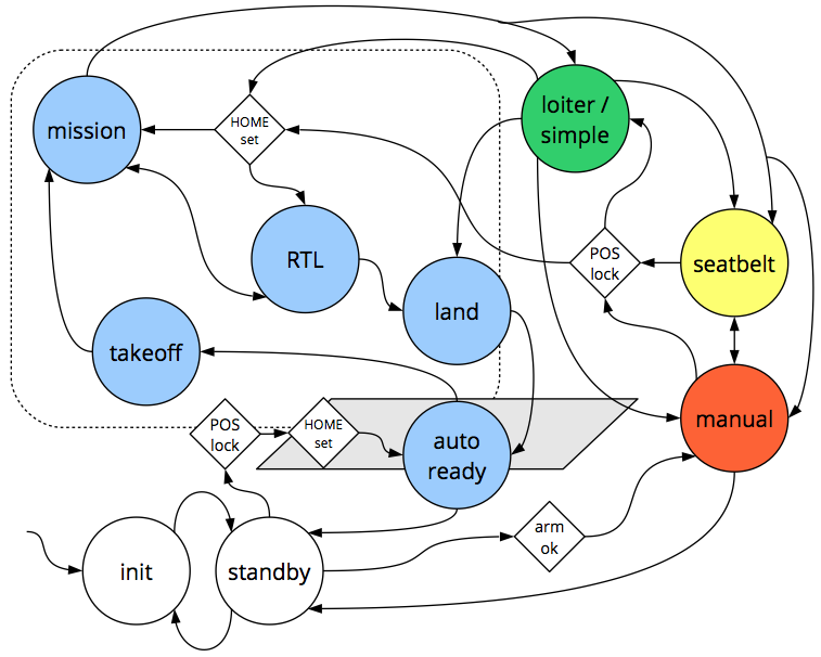
One important practical disadvantage of FSMs is that their complexity does not scale well with system complexity, and, generally speaking, it can be time consuming and challenging to design FSMs for practical robotic systems. To reduce complexity as much as possible, we must carefully choose the appropriate set of states to represent the system, and even with a well-defined set of states the interactions and transitions between states can be complex and hard to specify. For example, Figure 16.3 shows a graphical representation of the FSM for the popular open source flight software PX4^†^†margin: PX4 is a flight control software for drones and other unmanned vehicles. See https://px4.io/ for more information. . Specifying the full behavior for a system like this can lead to a complex FSM, even if there are not very many states.

Refer to caption — Figure 16.3: A graphical representation of the FSM for PX4. We can see that even for a relatively small number of states, the FSM is quite complex in order to model the full behavior of the system. Image retrieved from diydrones.com.

At a high level, three complementary techniques help manage this complexity:

•

State Minimization, which merges behaviorally equivalent states to remove redundancy.
•

Hierarchical State Machines, which allow states to be nested within other states to create a hierarchy of states.
•

Composition, where larger state machines are built from smaller, simpler state machines.

16.2.1 State Minimization

A standard way to reduce an FSM without changing its input–output behavior is partition refinement. Two states are equivalent if, for every input string, they produce the same output sequence (Mealy) or the same state outputs (Moore) and transition to equivalent states. Partition refinement starts from a coarse partition—states that are immediately distinguishable by their outputs—and repeatedly refines the blocks by splitting states whose next states fall into different blocks for some input. When the process reaches a fixed point, merging the states within each block yields a minimal machine with the same behavior. We provide an example of this procedure in Example 16.2.1.

Example 16.2.1 (Finite State Machine State Reduction).

Consider a FSM that detects the input sequences 010 or 110. Table 16.1 lists the next-state function and the output function for each state and input. We can see that the states are the partial sequences and a Reset state, $S\coloneqq\{0,1,00,01,10,11,\text{Reset}\}$ , the inputs are $I\coloneqq\{0,1\}$ , and the outputs are the booleans $O\coloneqq\{\text{True},\text{False}\}$ that indicate if the sequence 010 or 110 has been created. For example, if the current partial sequence is 01 and a 0 is input, the next state will be the Reset state and the output will be True.

State, $s$	$n(s,0)$	$n(s,1)$	$o(s,0)$	$o(s,1)$
Reset	0	1	False	False
0	00	01	False	False
1	10	11	False	False
00	Reset	Reset	False	False
01	Reset	Reset	True	False
10	Reset	Reset	False	False
11	Reset	Reset	True	False

Table 16.1: FSM for a sequence detector that accepts digits 0 and 1 and outputs True if the sequences 010 or 110 are generated.

We can now simplify this FSM by removing redundant states. To do so, we begin with the initial partition that groups states based on their output behavior:

\begin{split}\{\text{Reset},0,1,00,10\}&:\text{always leads to a False output}% ,\\ \{01,11\}&:\text{does not always lead to False output}.\end{split}

We then further partition these sets based on the next-state function until we cannot make any further partitions. In the first step, we partition the set $\{\text{Reset},0,1,00,10\}$ into:

\begin{split}\{\text{Reset},00,10\}&:\text{cannot transition to \{01,11\}},\\ \{0,1\}&:\text{can transition to \{01,11\}},\end{split}

and then partition $\{\text{Reset},00,10\}$ into:

\begin{split}\{\text{Reset}\}&:\text{can transition to }\{0,1\},\\ \{00,10\}&:\text{cannot transition to }\{0,1\}.\end{split}

After applying the partition refinement procedure, the original seven states $\{0,\allowbreak 1,\allowbreak 00,\allowbreak 01,\allowbreak 10,\allowbreak 11,% \text{Reset}\}$ are reduced to four states, $S_{\text{new}}=\{\{01,11\},\allowbreak\{0,1\},\allowbreak\{00,10\},\allowbreak% \text{Reset}\}$ . The resulting machine, shown in Table 16.2, is therefore an equivalent^†^†margin: Equivalent here meaning it has the same input–output behavior. but reduced FSM.

State, $s$	$n(s,0)$	$n(s,1)$	$o(s,0)$	$o(s,1)$
Reset	{0,1}	{0,1}	False	False
{0,1}	{00,10}	{01,11}	False	False
{00,10}	Reset	Reset	False	False
{01,11}	Reset	Reset	True	False

Table 16.2: Reduced FSM for the 010 or 110 sequence detector.

16.2.2 Hierarchical FSMs

In some cases there are states that are not strictly equivalent but are closely related in behavior. A common way to manage such structure is to use hierarchical finite state machines (HFSMs), also known as Statecharts⁸8. Harel, D. “Statecharts: A visual formalism for complex systems.” Science of Computer Programming 8(3), 231–274, 1987.. HFSMs introduce super-states^†^†margin: Also called composite states. that group together related states into a higher-level state, and generalized transitions that allow transitions to and from these super-states. This reduces diagram clutter and mitigates state explosion by allowing behavior to be factored and reused across related modes. Compared to flat FSMs, HFSMs support modularity, abstraction, and reuse of shared transitions at higher levels of the hierarchy. Harel (1987)¹1. Harel, D. “Statecharts: A visual formalism for complex systems.” Science of Computer Programming 8(3), 231–274, 1987. and Alur (2015)²2. Alur, R. Algorithms for Decision Making. MIT Press, 2015. provide an in-depth treatment of hierarchical FSMs, including formal definitions, semantics, and algorithms for analysis and verification.

16.2.3 Compositions

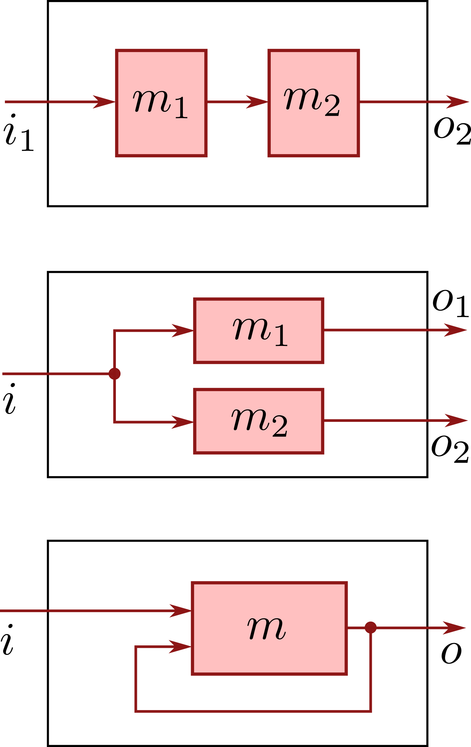
We can also compose individual state machines in a variety of ways depending on their input/output behavior, including cascade compositions, parallel compositions, and feedback compositions.

An example of each of these composition types is shown in Figure 16.4.

Cascade (serial) composition.

Let $M_{1}=(S_{1},I_{1},O_{1},n_{1},o_{1},s_{1,0})$ and $M_{2}=(S_{2},\allowbreak I_{2},\allowbreak O_{2},\allowbreak n_{2},\allowbreak o% _{2},\allowbreak s_{2,0})$ be two FSMs and assume a wiring map $\rho:O_{1}\to I_{2}$ (often $\rho$ is the identity after renaming). The cascade composition $M=M_{2}\circ_{\rho}M_{1}$ is defined as the FSM $M=(S,I,O,n,o,s_{0})$ where:

$\displaystyle S$	$\displaystyle=S_{1}\times S_{2},$	(16.1)
$\displaystyle I$	$\displaystyle=I_{1},$
$\displaystyle O$	$\displaystyle=O_{2},$
$\displaystyle n((s_{1},s_{2}),i)$	$\displaystyle=(n_{1}(s_{1},i),n_{2}(s_{2},\rho(o_{1}(s_{1},i)))),$
$\displaystyle o((s_{1},s_{2}),i)$	$\displaystyle=o_{2}(s_{2},\rho(o_{1}(s_{1},i))),$
$\displaystyle s_{0}$	$\displaystyle=(s_{1,0},s_{2,0}).$

Intuitively, $M_{1}$ processes the external input $i$ and produces an output $o_{1}(s_{1},i)$ , which is then fed into $M_{2}$ as input via the wiring map $\rho$ .

Parallel (synchronous) composition.

Parallel compositions combine two FSMs that share the same input alphabet and operate simultaneously on the same input. Let $M_{1}=(S_{1},I,O_{1},n_{1},o_{1},s_{1,0})$ and $M_{2}=(S_{2},I,O_{2},n_{2},o_{2},s_{2,0})$ be two FSMs with the same input alphabet $I$ . The parallel composition $M=M_{1}\parallel M_{2}$ is defined as the FSM $M=(S,I,O,n,o,s_{0})$ where:

$\displaystyle S$	$\displaystyle=S_{1}\times S_{2},$	(16.2)
$\displaystyle I$	$\displaystyle=I,$
$\displaystyle O$	$\displaystyle=O_{1}\times O_{2},$
$\displaystyle n((s_{1},s_{2}),i)$	$\displaystyle=(n_{1}(s_{1},i),n_{2}(s_{2},i)),$
$\displaystyle o((s_{1},s_{2}),i)$	$\displaystyle=(o_{1}(s_{1},i),o_{2}(s_{2},i)),$
$\displaystyle s_{0}$	$\displaystyle=(s_{1,0},s_{2,0}).$

Feedback composition.

Feedback compositions connect (part of) an FSM’s output back to its input, creating a closed-loop system. The closed-loop machine is well-defined if the induced equations have a unique solution for the input given the output. Otherwise, the feedback composition is said to be ill-formed.

16.3 Limitations of Finite State Machines

FSMs provide a clear, simple, and formally verifiable framework for discrete decision-making, which makes them attractive for implementing basic robot behaviors. However, their effectiveness as the primary control architecture for complex autonomous robots is fundamentally limited. Although the architectural techniques discussed in Section 16.2 can alleviate some practical issues, they do not address the core limitations of the FSM paradigm. In practice, FSMs are best suited to highly structured environments in which the set of relevant situations and required responses is small, predictable, and can be exhaustively anticipated by a designer.

As the complexity of a robot’s task and environment increases, FSM-based systems become difficult to scale. The number of states required to accurately represent the system can grow combinatorially with the number of factors that influence decision-making, including both the robot’s internal operating mode and aspects of the external world such as object configurations or the behavior of other agents.

FSMs also tend to exhibit brittle behavior when deployed outside the situations explicitly anticipated by their designers. Because all transitions and responses must be hand-specified, the robot can only react meaningfully to inputs for which logic has been defined in advance. When confronted with novel objects, unmodeled environmental changes, or unexpected sensor readings, the FSM lacks a mechanism for reasoning about new information or generalizing from prior experience. As a result, reliable performance is difficult to achieve in open-ended or dynamic environments without extensive manual engineering.

Another limitation of FSMs is the absence of an intrinsic notion of optimality. Standard FSMs describe which behaviors are permissible, but they do not provide a formal way to evaluate or compare alternative actions in terms of cost, reward, or long-term objectives. While it is possible to encode heuristically chosen preferences through careful state and transition design, the FSM framework itself does not support principled decision-making based on the optimization of a defined performance criterion. The system simply executes the logic that has been predefined.

Finally, the deterministic nature of FSMs makes them a poor match for the uncertainty inherent in real-world robotics. Sensor measurements are noisy, action outcomes are often stochastic, and the robot’s internal representation of the world is typically incomplete or approximate. Although designers can introduce states that qualitatively represent uncertainty, such as hypothesized or likely conditions, FSMs do not provide a principled mechanism for updating beliefs or making decisions based on probabilistic information.

Taken together, these limitations—poor scalability, sensitivity to unanticipated situations, and the inability to reason explicitly about optimality and uncertainty—motivate the use of more expressive decision-making frameworks. In the next chapters, we will introduce decision-making frameworks which support optimization under stochastic dynamics, as well as extensions that address partial observability, and learning-based approaches that allow robots to acquire complex behaviors from data rather than relying solely on manual specification.

16.4 Summary

In this chapter, we introduced finite state machines as a mathematical model for systems with discrete states and transitions. We defined the components of an FSM, including states, input and output alphabets, state transition functions, and output functions. We explored how FSMs can be represented using state diagrams and transition tables, providing visual and tabular representations of their behavior. Recognizing that FSMs can rapidly grow in complexity, we discussed three architectural strategies for managing this complexity: state minimization, hierarchical finite state machines, and mechanisms for composing FSMs.

To learn more.

For a rigorous and comprehensive introduction to finite state machines within the broader context of computation, a classic resource is the textbook by Sipser (1996)³3. Sipser, M. Introduction to the Theory of Computation. International Thomson Publishing, 1996. on the theory of computation. The seminal paper by Harel (1987)⁴4. Harel, D. “Statecharts: A visual formalism for complex systems.” Science of Computer Programming 8(3), 231–274, 1987. is essential reading for a deep understanding of hierarchical FSMs, which it introduced as Statecharts. For a more modern and formal textbook treatment of hybrid systems, including hierarchical and concurrent state machines, see Alur (2015)⁵5. Alur, R. Algorithms for Decision Making. MIT Press, 2015.. Finally, for the application of these concepts in the wider context of AI for robotics, we refer to the course by Kaelbling et al. (2011)⁶6. Kaelbling, L., White, J., Abelson, H., Freeman, D., Lozano-Pérez, T., Chuang, I. 6.01SC: Introduction to Electrical Engineering and Computer Science I. MIT OpenCourseWare, 2011..

16.5 Exercises

The starter code for the exercises provided below is available online through GitHub. To get started, download the code by running in a terminal window:

⬇

git clone https://github.com/StanfordASL/pora-exercises.git

We denote Problems requiring hand-written solutions and coding in Python with and , respectively.

Problem 1: State Machine

In this problem, you will create a finite state machine for a simple autonomous machine of your choice. For the system of your choice, define the set of states $S$ , the input alphabet $I$ , the output alphabet $O$ , the next–state function $n:S\times I\to S$ , and the initial state $s_{0}\in S$ . Define the output function using the Mealy machine convention. Draw a diagram of the state machine similar to Figure 16.2.