Sequential Decision Making and Dynamic Programming

In the referenced item, we introduced finite state machines as a structured and explicit way to model the logical flow of a robot’s behavior, allowing us to hand-design a set of rules that govern its actions in response to events. For well-defined tasks with a limited number of states, a carefully crafted finite state machine is an effective and interpretable way to implement a robot’s decision-making logic. However, the very structure that makes finite state machines clear also imposes fundamental limitations, especially as the complexity and uncertainty of the robot’s environment grow.

This chapter introduces a more general, optimization-based framework that directly addresses these limitations. Rather than manually specifying decision rules, we formulate decision-making as a mathematical optimization problem, allowing optimal actions to be computed automatically for complex, multi-step tasks, even under uncertainty. The central computational tool explored in this chapter is dynamic programming, a powerful algorithmic paradigm for solving sequential decision-making problems. Dynamic programming operates by decomposing complex, long-horizon problems into a sequence of simpler, nested subproblems that can be solved efficiently. As we will see, it also provides the theoretical foundation for modern learning-based approaches like reinforcement learning (the referenced item) and imitation learning (the referenced item).

We begin in Section 17.1 by applying dynamic programming to deterministic decision-making problems, where the robot’s actions have certain and predictable outcomes. We then extend this framework in Section 17.2 to stochastic decision-making problems, specifically Markov decision processes (MDPs), which explicitly account for uncertainty in the environment. Finally, in Section 17.3, we discuss the limitations of classical dynamic programming methods, thereby motivating the learning-based approaches introduced in later chapters.

17.1 Deterministic Sequential Decision Making

We begin our study of dynamic programming by introducing a simple, yet extremely general, formulation of sequential decision making. Despite its apparent simplicity, this formulation captures a wide range of problems arising in robotics, control, operations research, and artificial intelligence. We first consider the deterministic case, where the outcome of each action is fully predictable, before addressing stochasticity in the next section.

In this formulation, time is modeled as a sequence of discrete stages at which decisions are made. That is, we consider a discrete-time setting^†^†margin: The continuous-time counterpart to dynamic programming is the Hamilton-Jacobi-Bellman (HJB) equation. While the HJB equation is beyond the scope of this chapter, we refer interested readers to Bertsekas (2000)¹1. Bertsekas, D. Dynamic Programming and Optimal Control. Athena Scientific, 2000. for a comprehensive treatment of continuous-time decision-making. , where the evolution of the system is described by a difference equation of the form:

\bm{x}_{t+1}=f_{t}(\bm{x}_{t},\bm{u}_{t}),\quad t=0,\dots,T-1,

(17.1)

where $\bm{x}_{t}\in\mathbb{R}^{n}$ denotes the system state at time step $t$ , $\bm{u}_{t}\in\mathbb{R}^{m}$ is the control applied at that step, and $f_{t}$ specifies how the state evolves. The integer $T$ defines a finite planning horizon.

At each time step, not all controls may be available. We therefore associate with each state $\bm{x}_{t}$ a set of admissible controls, denoted by $\mathcal{U}(\bm{x}_{t})$ , and impose the constraint:

\bm{u}_{t}\in\mathcal{U}(\bm{x}_{t}),\quad t=0,\dots,T-1.

(17.2)

No particular structure is assumed for $\mathcal{U}(\bm{x}_{t})$ . Depending on the application, it may be a finite set of discrete actions, a continuous region of allowable inputs, or a state-dependent subset encoding physical, logical, or resource limitations.

The objective of the decision making problem is specified through an additive cost function defined over the planning horizon:

J(\bm{x}_{0},\bm{u}_{0},\dots,\bm{u}_{T-1})=g_{T}(\bm{x}_{T})+\sum_{t=0}^{T-1}% g_{t}(\bm{x}_{t},\bm{u}_{t}),

(17.3)

where $g_{t}$ represents the stage cost incurred at time $t$ and $g_{T}$ is a terminal cost applied to the final state. The additivity of the cost over time is a central structural assumption: it is this property that enables the decomposition of the problem into simpler subproblems, which lies at the heart of dynamic programming. No assumptions are made regarding smoothness, convexity, or time invariance of the cost functions.

The deterministic sequential decision making problem can be formally defined as follows:

Definition 17.1 (Deterministic Sequential Decision Making Problem).

Given the discrete-time system (Equation 17.1), the control constraints (Equation 17.2), and the additive cost function (Equation 17.3), the deterministic sequential decision making problem can be stated as the following optimization problem:

\begin{split}J^{*}(\bm{x}_{0})=\underset{\bm{u}_{t},\>\>t=0,\dots,T-1}{\text{% minimize}}&\quad g_{T}(\bm{x}_{T})+\sum_{t=0}^{T-1}g_{t}(\bm{x}_{t},\bm{u}_{t}% ),\\ \text{subject to}&\quad\bm{x}_{t+1}=f_{t}(\bm{x}_{t},\bm{u}_{t}),\quad t=0,% \dots,T-1,\\ &\quad\bm{u}_{t}\in\mathcal{U}(\bm{x}_{t}),\quad t=0,\dots,T-1.\end{split}

(17.4)

As we will see throughout the remainder of this chapter, the central goal of dynamic programming is to compute a solution to Problem (Equation 17.4) in the form of an optimal closed-loop control policy:

\begin{split}\pi=&\{\pi_{0},\ldots,\pi_{T-1}\},\\ \bm{u}_{t}^{*}=&\pi_{t}^{*}(\bm{x}_{t}),\quad t=0,\dots,T-1,\end{split}

(17.5)

where the policy $\pi$ denotes a sequence of functions $\pi_{t}$ mapping any state $\bm{x}_{t}$ into a control $\bm{u}_{t}$ ^†^†margin: In the deterministic setting considered here, the system evolution is fully predictable, and closed-loop and open-loop optimal solutions therefore coincide. The true advantages of closed-loop policies emerge mainly in the stochastic setting, which we address in the next section. .

In Chapter 3, we were able to derive closed-loop control laws primarily by exploiting strong structural assumptions, such as linear system dynamics, quadratic cost functions, or special system properties like differential flatness. While these assumptions yield elegant and computationally efficient solutions, they substantially limit the range of problems that can be addressed. Dynamic programming offers a fundamentally different approach. Rather than relying on restrictive structural properties, it exploits only the sequential nature of the decision-making process and the additive structure of the cost function, thereby providing a systematic framework for computing optimal closed-loop policies for a much broader class of systems, including those with nonlinear dynamics and non-quadratic costs.

In what follows, we will explore how dynamic programming can be employed to solve the deterministic decision making problem defined above through the so-called principle of optimality.

17.1.1 The Principle of Optimality

The dynamic programming approach to sequential decision making rests on a very simple, yet powerful, idea, known as the principle of optimality^†^†margin: Often referred to as Bellman’s principle of optimality. . Despite its simplicity, this principle is the key that transforms an otherwise intractable optimization problem into one that can be solved efficiently through recursive decomposition.

At a high level, the principle of optimality expresses the following insight. Suppose that a policy is optimal for a given decision making problem. Then, if we consider any intermediate time and the state reached at that time while following this policy, the remaining decisions prescribed by the policy must themselves be optimal for the subproblem that starts from that state. In other words, any tail segment of an optimal policy must itself be optimal for the corresponding tail subproblem.

The intuitive justification for this principle is straightforward. If the remaining decisions after some time were not optimal for the corresponding tail subproblem, then we could replace them with a better alternative and thereby reduce the total cost. This would contradict the assumption that the original policy was optimal. Thus, optimal policies must be composed of optimal solutions to all of their tail subproblems.

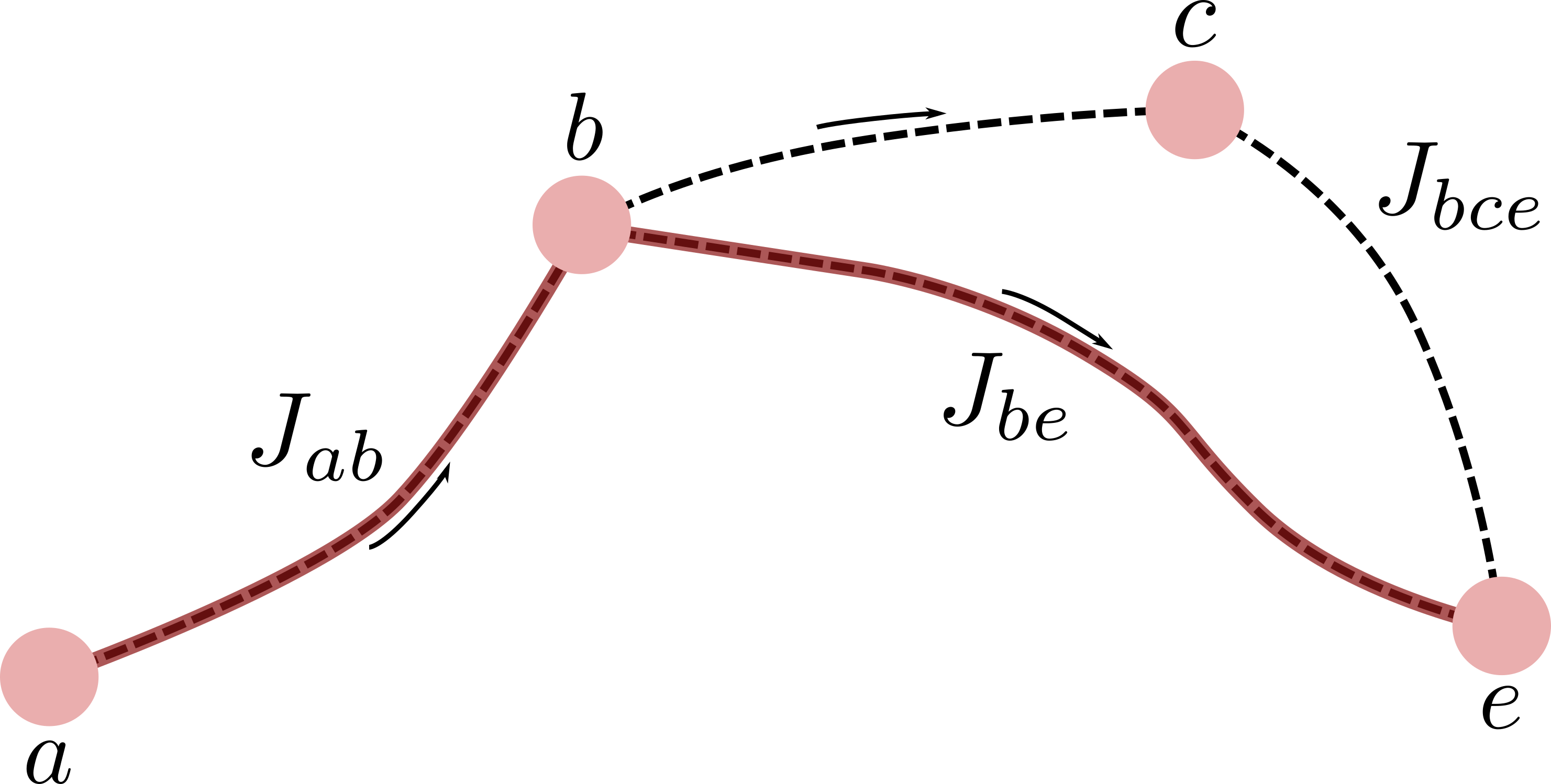
This idea is most easily visualized in shortest-path problems, as illustrated in Figure 17.1. If the optimal path from a starting point $a$ to a destination $e$ passes through an intermediate point $b$ , then the portion of the path from $b$ to $e$ must itself be optimal among all paths that start at $b$ . Otherwise, a shorter path from $b$ to $e$ could be substituted, yielding a shorter overall path from $a$ to $e$ .

Refer to caption — Figure 17.1: Illustration of the principle of optimality for a shortest-path problem. If the path $a\rightarrow b\rightarrow e$ is optimal from $a$ to $e$ , then the subpath $b\rightarrow e$ must be optimal when starting from $b$ . Adapted from Kirk (2004)²2. Kirk, D. E. *Optimal Control Theory: An Introduction*. Dover Publications, 2004..

We now state the principle of optimality formally for deterministic decision making problems.

Theorem 17.2 (Principle of Optimality (Deterministic Case)).

Let $\{\bm{u}_{0}^{*},\bm{u}_{1}^{*},\dots,\bm{u}_{T-1}^{*}\}$ be an optimal control sequence to the deterministic decision making problem defined by Problem 17.4 with initial condition $\bm{x}^{*}_{0}$ , and let $\{\bm{x}_{0}^{*},\bm{x}_{1}^{*},\dots,\bm{x}_{T}^{*}\}$ denote the corresponding optimal state trajectory. Then, for any time $t\in\{0,\dots,T-1\}$ , the truncated control sequence $\{\bm{u}_{t}^{*},\dots,\bm{u}_{T-1}^{*}\}$ is optimal for the subproblem that starts from state $\bm{x}_{t}^{*}$ at time $t$ and minimizes the tail cost:

J_{\text{tail}}(\bm{x}_{t},\bm{u}_{t},\dots,\bm{u}_{T-1})=g_{T}(\bm{x}_{T})+% \sum_{i=t}^{T-1}g_{i}(\bm{x}_{i},\bm{u}_{i}),

subject to the same system dynamics and control constraints, over the horizon $t$ to $T$ .

The principle of optimality suggests that an optimal policy can be constructed by solving a sequence of smaller subproblems. One may first solve the tail subproblem involving only the final stage, then extend this solution to the tail subproblem involving the last two stages, and continue in this manner until an optimal policy for the entire horizon is obtained. The dynamic programming algorithm is based precisely on this idea: it proceeds backward in time, solving tail subproblems of increasing length by reusing solutions to shorter tail subproblems.

Example 17.1.1 (Shortest-Path Problem).

Consider the deterministic shortest-path problem shown in Figure 17.2, where the objective is to find an optimal path from point $b$ to point $f$ . Suppose that the optimal costs from points $c$ , $d$ , and $e$ to $f$ are already known.

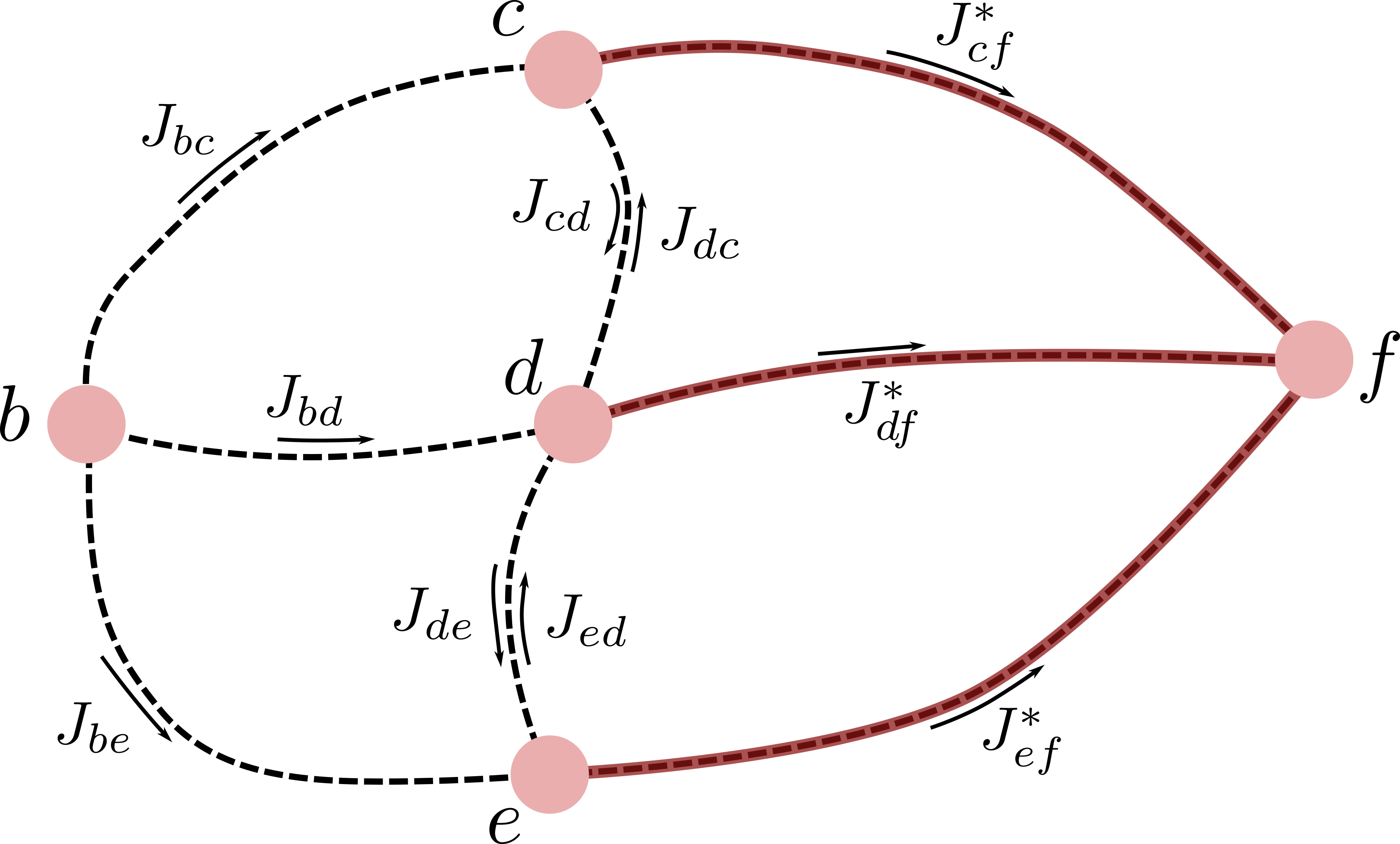
A brute-force approach would require evaluating all possible paths from $b$ to $f$ , including:

\begin{split}\{b\rightarrow c\rightarrow f,\;b\rightarrow c\rightarrow d% \rightarrow f,\;b\rightarrow c\rightarrow d\rightarrow e\rightarrow f,\;b% \rightarrow d\rightarrow c\rightarrow f,\;b\rightarrow d\rightarrow f,\\ b\rightarrow d\rightarrow e\rightarrow f,\;b\rightarrow e\rightarrow d% \rightarrow c\rightarrow f,\;b\rightarrow e\rightarrow d\rightarrow f,\;b% \rightarrow e\rightarrow f\}.\end{split}

By exploiting the principle of optimality, we know that any optimal path from $b$ to $f$ must consist of an immediate step from $b$ to one of its neighboring points ( $c$ , $d$ , or $e$ ), followed by an optimal path from that neighboring point to $f$ . Thus, only three candidate paths need to be evaluated:

b\rightarrow c\rightarrow f,\quad b\rightarrow d\rightarrow f,\quad b% \rightarrow e\rightarrow f,

where the optimal path can be found by selecting the minimum-cost path among:

\{J_{bc}+J^{*}_{cf},\;J_{bd}+J^{*}_{df},\;J_{be}+J^{*}_{ef}\}.

This simple example illustrates the central idea underlying dynamic programming, where optimal tail costs are reused to efficiently construct optimal solutions to larger problems. We now formalize this idea into a systematic algorithm for solving sequential decision making problems.

17.1.2 The Dynamic Programming Algorithm

The principle of optimality provides a powerful structural property of optimal solutions, but by itself it does not specify how such solutions should be computed. Dynamic programming turns this structural insight into a concrete computational procedure to find optimal control policies.

Rather than attempting to find an optimal control sequence over the entire horizon at once, dynamic programming proceeds by solving a sequence of smaller subproblems backward in time. This motivates the introduction of the so-called cost-to-go function. For each time $t\in\{0,\dots,T\}$ and each state $\bm{x}_{t}$ , define the optimal cost-to-go $J_{t}^{*}(\bm{x}_{t})$ as the minimum achievable cost when the system starts from state $\bm{x}_{t}$ at time $t$ and evolves optimally until the terminal time $T$ . By definition, the cost-to-go at time $T$ coincides with the terminal cost:

J_{T}^{*}(\bm{x}_{T})=g_{T}(\bm{x}_{T}),\quad\forall\bm{x}_{T}\in\mathcal{X},

since no further decisions remain to be made after time $T$ .

The principle of optimality implies that the optimal cost-to-go functions satisfy a recursive relationship, where the cost-to-go at time $t$ can be expressed in terms of the stage cost at time $t$ and the cost-to-go at time $t+1$ :

J_{t}^{*}(\bm{x}_{t})=\min_{\bm{u}_{t}\in\mathcal{U}(\bm{x}_{t})}\Bigl{[}g_{t}% (\bm{x}_{t},\bm{u}_{t})+J_{t+1}^{*}\bigl{(}f_{t}(\bm{x}_{t},\bm{u}_{t})\bigr{)% }\Bigr{]},\qquad t=0,\dots,T-1.

(17.6)

This equation, often referred to as the Bellman equation, expresses the global optimization problem in terms of a local minimization combined with the optimal solution of a shorter-horizon problem.

In practice, the dynamic programming algorithm leverages the Bellman equation to compute the optimal cost-to-go functions via a backward-in-time recursion, as summarized in Algorithm 1. Starting from the known terminal cost $J_{T}^{*}$ , one computes $J_{T-1}^{*}$ , then $J_{T-2}^{*}$ , and so on, until $J_{0}^{*}$ is obtained. At each stage of this backward recursion, the optimal tail cost is computed for every state in the state space. The result is a collection of functions $\{J_{t}^{*}(\cdot)\}_{t=0}^{T}$ that completely characterize the optimal performance of the system from any state and time.

J^{*}_{T}(\bm{x}_{T})=g_{T}(\bm{x}_{T}),

for all

\bm{x}_{T}\in\mathcal{X}

for $t=T-1$ to $0$ do

J^{*}_{t}(\bm{x}_{t})=\min_{\bm{u}_{t}\in\mathcal{U}(\bm{x}_{t})}\Bigl{[}g_{t}%(\bm{x}_{t},\bm{u}_{t})+J_{t+1}^{*}\bigl{(}f_{t}(\bm{x}_{t},\bm{u}_{t})\bigr{)%}\Bigr{]},\qquad

for all

\bm{x}_{t}\in\mathcal{X}

return

J^{*}_{0}(\cdot),\dots,J^{*}_{T}(\cdot)

Algorithm 1 Dynamic Programming (Deterministic)

Once the cost-to-go functions have been computed, the optimal control at each time step is obtained by minimizing the sum of the immediate cost and the optimal cost-to-go of the resulting next state:

\bm{u}_{t}^{*}=\operatorname*{arg\,min}_{\bm{u}_{t}\in\mathcal{U}(\bm{x}_{t}^{% *})}\Bigl{[}g_{t}(\bm{x}_{t}^{*},\bm{u}_{t})+J_{t+1}^{*}\bigl{(}f_{t}(\bm{x}_{% t}^{*},\bm{u}_{t})\bigr{)}\Bigr{]}.

The system is then propagated to the next state $\bm{x}_{t+1}^{*}=f_{t}(\bm{x}_{t}^{*},\bm{u}_{t}^{*})$ , and the process is repeated until the terminal time $T$ is reached. Conceptually, the backward pass computes the optimal cost-to-go functions of every tail subproblem, while the forward pass uses these functions to compute the actions that realize these optimal costs.

Although dynamic programming yields an exact solution to the deterministic decision making problem, its direct application is often limited by computational considerations. The backward recursion requires evaluating the Bellman equation for every possible state at every time step, which may be infeasible when the state space is continuous or very large. Discretization of the state space may render the algorithm implementable, but even then the computational burden can grow rapidly with the dimension of the state. These challenges motivate the development of approximate methods that retain the conceptual framework of dynamic programming while relaxing its computational demands.

Despite these practical limitations, dynamic programming occupies a central role in sequential decision making. It provides the canonical solution method for finite-horizon problems, offers a precise interpretation of optimality through cost-to-go functions, and serves as the conceptual foundation for a wide range of learning-based control algorithms.

Example 17.1.2 (Grid Navigation).

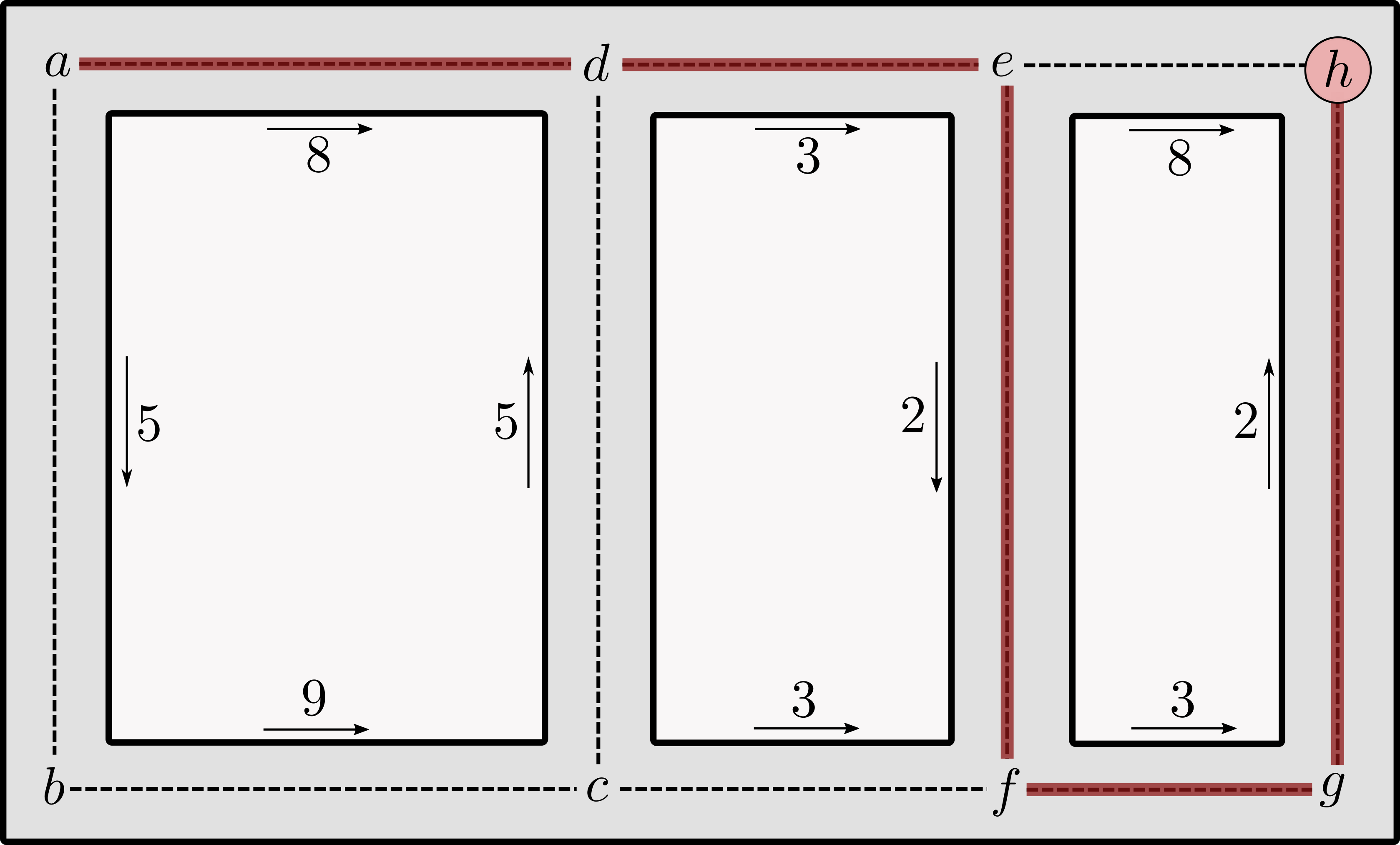
Consider the environment shown in Figure 17.3, where the objective is to move from point $a$ to point $h$ while incurring the minimum possible cost. The state $\bm{x}=\{a,b,c,d,e,f,g,h\}$ corresponds to the agent’s current location on the grid, and the available control actions at each state are encoded by the arrows indicating allowable directions of travel. For example, at point $c$ the agent may move either right or up, but not left or down. Each directed edge is associated with a nonnegative traversal cost, as shown in the figure.

We treat point $h$ as a terminal state with zero terminal cost, so that:

J^{*}_{T}(h)=0,

and we allow the agent to remain at $h$ at zero cost once it is reached. The dynamic programming recursion is initialized at this terminal condition and proceeds backward in time, successively computing the optimal cost-to-go for states that can reach $h$ within an increasing number of steps.

At the first backward step, corresponding to one step from the terminal time, only states that can transition directly to $h$ are relevant. These are the points $e$ and $g$ , together with $h$ itself. The optimal costs-to-go are obtained by adding the immediate transition cost to the terminal cost:

\begin{split}J^{*}_{T-1}(h)&=0+J^{*}_{T}(h)=0,\quad u^{*}_{T-1}(h)=\text{stay}% ,\\ J^{*}_{T-1}(e)&=8+J^{*}_{T}(h)=8,\quad u^{*}_{T-1}(e)=\text{right},\\ J^{*}_{T-1}(g)&=2+J^{*}_{T}(h)=2,\quad u^{*}_{T-1}(g)=\text{up}.\\ \end{split}

At the next step of the recursion, states such as $d$ and $f$ become relevant, since they can reach $h$ in two steps. Their optimal costs-to-go are computed by adding the immediate cost of moving to $e$ or $g$ and then using the previously computed one-step tail costs:

\begin{split}J^{*}_{T-2}(d)=3+J^{*}_{T-1}(e)=11,\quad&u^{*}_{T-2}(d)=\text{% right},\\ J^{*}_{T-2}(f)=3+J^{*}_{T-1}(g)=5,\quad&u^{*}_{T-2}(f)=\text{right}.\\ \end{split}

At this point, the cost-to-go values represent the optimal cost of reaching $h$ in at most two steps from each of the states $\{d,e,f,g\}$ .

As the recursion continues, additional states enter the computation, and some states acquire multiple feasible paths to the terminal state. For example, at the next backward step, state $e$ may either move directly to $h$ or move downward to $f$ and then proceed optimally from there. The Bellman equation automatically selects the cheaper of these alternatives:

J^{*}_{T-3}(e)=\min\{8+J^{*}_{T-2}(h),\,2+J^{*}_{T-2}(f)\}=7,\quad u^{*}_{T-3}% (e)=\text{down}.

Similarly, the other relevant states at this step are updated as follows:

\begin{split}J^{*}_{T-3}(g)=2,\quad&u^{*}_{T-3}(g)=\text{up},\\ J^{*}_{T-3}(d)=3+J^{*}_{T-2}(e)=11,\quad&u^{*}_{T-3}(d)=\text{right},\\ J^{*}_{T-3}(f)=5,\quad&u^{*}_{T-3}(f)=\text{right},\\ J^{*}_{T-3}(a)=8+J^{*}_{T-2}(d)=19,\quad&u^{*}_{T-3}(a)=\text{right},\\ J^{*}_{T-3}(c)=\min\{5+J^{*}_{T-2}(d),\>3+J^{*}_{T-2}(f)\}=8,\quad&u^{*}_{T-3}% (c)=\text{right}.\end{split}

At this stage, we see that the goal $h$ is reachable from $a$ in three time steps on path $a\rightarrow d\rightarrow e\rightarrow h$ , and that we would incur a cost of 19.

Extending the horizon further allows the algorithm to discover lower-cost paths that take advantage of additional intermediate states. In particular, the recursion continues one more step to yield:

\begin{split}J^{*}_{T-4}(e)=7,\quad&u^{*}_{T-4}(e)=\text{down},\\ J^{*}_{T-4}(g)=2,\quad&u^{*}_{T-4}(g)=\text{up},\\ J^{*}_{T-4}(d)=3+J^{*}_{T-3}(e)=10,\quad&u^{*}_{T-4}(d)=\text{right},\\ J^{*}_{T-4}(f)=5,\quad&u^{*}_{T-4}(f)=\text{right},\\ J^{*}_{T-4}(a)=8+J^{*}_{T-3}(d)=19,\quad&u^{*}_{T-4}(a)=\text{right},\\ J^{*}_{T-4}(c)=\min\{5+J^{*}_{T-3}(d),\>3+J^{*}_{T-3}(f)\}=8,\quad&u^{*}_{T-4}% (c)=\text{right},\\ J^{*}_{T-4}(b)=9+J^{*}_{T-3}(c)=17,\quad&u^{*}_{T-4}(b)=\text{right}.\\ \end{split}

Finally, extending the horizon one last time allows the algorithm to find the optimal path from the initial state $a$ to the goal state $h$ , corresponding to the path $a\rightarrow d\rightarrow e\rightarrow f\rightarrow g\rightarrow h$ , with total cost 18:

\begin{split}J^{*}_{T-5}(e)=7,\quad&u^{*}_{T-5}(e)=\text{down},\\ J^{*}_{T-5}(g)=2,\quad&u^{*}_{T-5}(g)=\text{up},\\ J^{*}_{T-5}(d)=10,\quad&u^{*}_{T-5}(d)=\text{right},\\ J^{*}_{T-5}(f)=5,\quad&u^{*}_{T-5}(f)=\text{right},\\ J^{*}_{T-5}(a)=\min\{8+J^{*}_{T-4}(d),\>5+J^{*}_{T-4}(b)\}=18,\quad&u^{*}_{T-5% }(a)=\text{right},\\ J^{*}_{T-5}(c)=\min\{5+J^{*}_{T-4}(d),\>3+J^{*}_{T-4}(f)\}=8,\quad&u^{*}_{T-5}% (c)=\text{right},\\ J^{*}_{T-5}(b)=9+J^{*}_{T-4}(c)=17,\quad&u^{*}_{T-5}(b)=\text{right}.\\ \end{split}

Several important features of dynamic programming are illustrated by this example. First, the algorithm does not search over complete paths from $a$ to $h$ . Instead, it incrementally builds optimal solutions by reusing previously computed tail costs. Second, the algorithm computes optimal costs and controls for all states, not just the initial state of interest. As a result, once the cost-to-go functions have been computed, optimal paths can be generated immediately from any starting point and for any horizon length. For example, starting from point $c$ with a horizon of three steps, the optimal path $c\rightarrow f\rightarrow g\rightarrow h$ and its associated cost of $8$ can be read off directly, without any additional computation.

17.2 Decision Making Under Uncertainty: Markov Decision Processes

The deterministic decision making framework developed in Section 17.1 provides a clean and powerful lens through which sequential decision making problems can be understood and solved. In realistic robotic systems, however, the environment is never perfectly known, and uncertainty is an intrinsic feature of physical interaction and perception. Sensor measurements are noisy, actuation is imperfect, and the environment may evolve in ways that cannot be modeled exactly or anticipated in advance. As a result, the evolution of the system state cannot be described deterministically, and decision quality must be evaluated in a statistical sense.

The goal of this section is to extend the deterministic sequential decision making problem in Definition 17.1 to explicitly account for such uncertainty. We begin by deriving a stochastic formulation of the sequential decision making problem that incorporates uncertainty into both the system dynamics and the cost structure, thereby introducing the framework of Markov decision processes (MDPs). This framework is a cornerstone of modern decision making under uncertainty, and will serve as a bridge to the learning-based methods developed in the referenced item and the referenced item. We then adapt the principle of optimality and the dynamic programming algorithm to this stochastic setting.

17.2.1 Problem Formulation

We begin by modifying the state transition model in (Equation 17.1) to include a stochastic disturbance:

\bm{x}_{t+1}=f_{t}(\bm{x}_{t},\bm{u}_{t},\bm{w}_{t}),\quad t=0,\dots,T-1,

(17.7)

where $\bm{w}_{t}$ denotes a stochastic disturbance at time $t$ . The disturbance $\bm{w}_{t}$ is assumed to be drawn from a known conditional probability distribution:

\bm{w}_{t}\sim p_{t}(\bm{w}_{t}\mid\bm{x}_{t},\bm{u}_{t}).

(17.8)

This assumption implies that the distribution of the next state depends only on the current state and action, and not on the full history of the system. This conditional independence assumption is an instance of the Markov property^†^†margin: Which we previously encountered in Chapter 11 in the context of Bayesian filtering. , which states that, given the present state and action, the future evolution of the system is independent of the past. Accordingly, the state $\bm{x}_{t}$ can be interpreted as a sufficient summary of all past information relevant for future decision making.

The admissible control constraints remain unchanged. At each time step, the control must satisfy:

\bm{u}_{t}\in\mathcal{U}(\bm{x}_{t}),\quad t=0,\dots,T-1,

(17.9)

where $\mathcal{U}(\bm{x}_{t})$ may encode physical limitations, logical constraints, or discrete action choices.

We also allow the instantaneous cost to depend explicitly on the disturbance:

g_{t}:\mathcal{X}\times\mathcal{U}\times\mathcal{W}\to\mathbb{R},\quad t=0,% \dots,T-1,

(17.10)

where $\mathcal{W}$ denotes the space of possible disturbance values.

Because the system evolution is now stochastic, performance can no longer be evaluated along a single trajectory. Instead, we measure performance in expectation. Specifically, given a policy $\pi=\{\pi_{0},\dots,\pi_{T-1}\}$ , we define the associated expected cost starting from an initial state $\bm{x}_{0}$ as:

J_{\pi}(\bm{x}_{0})=\mathbb{E}_{\bm{w}}\left[\,g_{T}(\bm{x}_{T})+\sum_{t=0}^{T% -1}g_{t}(\bm{x}_{t},\pi_{t}(\bm{x}_{t}),\bm{w}_{t})\,\right],

(17.11)

where the expectation is taken with respect to the joint distribution of the disturbance sequence $\{\bm{w}_{0},\dots,\bm{w}_{T-1}\}$ induced by the policy $\pi$ and the stochastic dynamics (Equation 17.7). This formulation corresponds to a risk-neutral objective, where policies are compared based on their average performance^†^†margin: While the expected cost formulation is the most common in the literature, alternative risk measures—such as worst-case performance or risk-sensitive criteria—can also be considered, but are beyond the scope of this chapter. .

We can now formally state the stochastic sequential decision making problem.

Definition 17.1 (Stochastic Sequential Decision Making Problem).

Given the stochastic dynamics (Equation 17.7), the control constraints (Equation 17.9), and the expected cost (Equation 17.11), the stochastic sequential decision making problem consists of computing an optimal policy:

\pi^{*}=\{\pi_{0}^{*},\dots,\pi_{T-1}^{*}\},

that solves:

\begin{split}J^{*}(\bm{x}_{0})=\underset{[}{\text{minimize}}\>\quad\pi]&% \mathbb{E}_{\bm{w}}\left[\,g_{T}(\bm{x}_{T})+\sum_{t=0}^{T-1}g_{t}(\bm{x}_{t},% \pi_{t}(\bm{x}_{t}),\bm{w}_{t})\,\right],\\ \text{subject to}\quad&\bm{x}_{t+1}=f_{t}(\bm{x}_{t},\bm{u}_{t},\bm{w}_{t}),% \quad t=0,\dots,T-1,\\ &\bm{u}_{t}=\pi_{t}(\bm{x}_{t})\in\mathcal{U}(\bm{x}_{t}),\>\>t=0,\dots,T-1.% \end{split}

(17.12)

This formulation is also known as a finite-horizon Markov decision process. It mirrors the deterministic problem in structure, differing only in the introduction of random disturbances and the use of expected cost as the performance criterion. As we will see next, this similarity allows us to extend the principle of optimality and dynamic programming methods to this stochastic setting^†^†margin: This problem formulation lies at the core of several disciplines, including optimal control, operations research, robotics, economics, and machine learning. As a result, it is common to encounter substantially different notation and terminology across communities, even when describing essentially the same underlying problem. In this chapter, we adopt notation that is standard in optimal control. In the next chapter, we will reintroduce the same problem using notation that is more common in the machine learning and reinforcement learning literature. For a broader discussion of the connections, overlaps, and distinctions among these perspectives, we refer the reader to Powell (2012)⁵5. Powell, W. B. “AI, OR and control theory: A Rosetta Stone for stochastic optimization.” In Princeton University, 2012.. .

17.2.2 Stochastic Decision Making with Dynamic Programming

As in the deterministic case, the key property that enables efficient solution methods for the stochastic sequential decision making problem is the principle of optimality. In this subsection, we first state the principle of optimality for the stochastic setting, and then show how it leads to a dynamic programming recursion for computing optimal policies.

Principle of Optimality.

In the stochastic setting, the core intuition behind the principle of optimality—that optimal policies can be constructed by composing optimal solutions to tail subproblems—remains valid. However, it must be formulated in terms of expected future cost. Because state transitions are random, it is no longer meaningful to reason in terms of a single “optimal trajectory”. Instead, policies are evaluated by the expected cumulative cost they induce under the stochastic elements in the system.

The crucial assumption that enables a recursive decomposition is the Markov property. Specifically, as introduced in Chapter 11, the Markov property ensures that the future evolution of the system depends only on the current state and action, and not on the full history leading up to that state. Consequently, the expected cost incurred from time $t$ onward depends only on $\bm{x}_{t}$ and the future actions selected by the policy.

Under this assumption, if a policy is optimal from the initial condition, then after reaching any intermediate state $\bm{x}_{t}$ , the remaining portion of that policy must still be optimal for the tail problem that starts at $\bm{x}_{t}$ . If this were not the case, the tail could be replaced by an alternative policy with strictly lower expected cost, thereby reducing the overall expected cost and contradicting the optimality of the original policy.

Formally, we can state the principle of optimality for the stochastic decision making problem as follows:

Theorem 17.2 (Principle of Optimality (Stochastic Case)).

Let $\pi^{*}=\{\pi_{0}^{*},\pi_{1}^{*},\dots,\pi_{T-1}^{*}\}$ be an optimal policy for the stochastic decision making problem defined in Problem 17.12. For any time $t$ and any state $\bm{x}_{t}$ that is reachable under $\pi^{*}$ , the tail policy $\{\pi_{t}^{*},\dots,\pi_{T-1}^{*}\}$ is an optimal policy for the tail subproblem that starts at time $t$ from state $\bm{x}_{t}$ and minimizes the expected cost:

J_{\pi}(\bm{x}_{t})=\mathbb{E}_{\bm{w}}\left[\,g_{T}(\bm{x}_{T})+\sum_{i=t}^{T% -1}g_{i}(\bm{x}_{i},\pi_{i}(\bm{x}_{i}),\bm{w}_{i})\,\right].

As in the deterministic case, this result implies that optimal policies can be constructed by solving a sequence of nested tail subproblems, with dynamic programming providing a systematic procedure for carrying out this backward construction, as we describe next.

Dynamic Programming.

The dynamic programming algorithm for the stochastic case closely mirrors its deterministic counterpart. It proceeds backward in time, starting from the terminal cost:

J_{T}^{*}(\bm{x}_{T})=g_{T}(\bm{x}_{T}),\quad\forall\bm{x}_{T}\in\mathcal{X},

and successively computing the optimal cost-to-go for earlier stages. At each step, the algorithm evaluates, for every state, the expected cost associated with each admissible control and selects the minimizing one. Similarly, the cost-to-go can be expressed recursively, yielding the (stochastic) Bellman equation:

J_{t}^{*}(\bm{x}_{t})=\min_{\bm{u}_{t}\in\mathcal{U}(\bm{x}_{t})}\mathbb{E}_{% \bm{w}}\left[g_{t}(\bm{x}_{t},\bm{u}_{t},\bm{w}_{t})+J_{t+1}^{*}\!\bigl{(}f_{t% }(\bm{x}_{t},\bm{u}_{t},\bm{w}_{t})\bigr{)}\right],\qquad t=0,\dots,T-1.

(17.13)

The resulting dynamic programming algorithm is summarized in Algorithm 2.

J_{T}^{*}(\bm{x})=g_{T}(\bm{x}),

for all

\bm{x}\in\mathcal{X}

for $t=T-1$ to $0$ do

J_{t}^{*}(\bm{x})=\underset{\bm{u}\in\mathcal{U}(\bm{x})}{\min}\mathbb{E}_{\bm%{w}}\left[g_{t}(\bm{x},\bm{u},\bm{w})+J_{t+1}^{*}(f_{t}(\bm{x},\bm{u},\bm{w}))%\right],

for all

\bm{x}\in\mathcal{X}

return

J_{0}^{*}(\cdot),\dots,J_{T}^{*}(\cdot)

Algorithm 2 Dynamic Programming (Stochastic Case)

Once the cost-to-go functions have been computed, an optimal policy is obtained by selecting:

\pi_{t}^{*}(\bm{x}_{t})=\operatorname*{arg\,min}_{\bm{u}_{t}\in\mathcal{U}(\bm% {x}_{t})}\mathbb{E}_{\bm{w}}\left[g_{t}(\bm{x}_{t},\bm{u}_{t},\bm{w}_{t})+J_{t% +1}^{*}\!\bigl{(}f_{t}(\bm{x}_{t},\bm{u}_{t},\bm{w}_{t})\bigr{)}\right].

(17.14)

Example 17.2.1 (Inventory Control).

Consider a simple inventory control problem in which the state $x_{t}\in\mathbb{N}$ denotes the available stock of an item at time $t$ . At each step, the decision maker chooses how many items to order, $u_{t}\in\mathbb{N}$ , before facing a random demand $w_{t}\in\mathbb{N}$ .

The system dynamics are given by:

x_{t+1}=\max\{0,\,x_{t}+u_{t}-w_{t}\},

which captures the fact that demand reduces inventory, restocking increases it, and inventory cannot go below zero. We impose the constraint:

x_{t}+u_{t}\leq 2,

so that the inventory capacity is limited to at most two units.

Demand is modeled as a discrete random variable with the following probability distribution:

p(w_{t}=0)=0.1,\quad p(w_{t}=1)=0.7,\quad p(w_{t}=2)=0.2.

We consider a finite horizon of $T=3$ steps and define the expected cost:

\mathbb{E}_{w}\left[\sum_{t=0}^{2}\bigl{(}u_{t}+(x_{t}+u_{t}-w_{t})^{2}\bigr{)% }\right],

which penalizes both ordering costs and the squared deviation between inventory and demand.

To solve this problem using dynamic programming, we first identify the state and control spaces:

\mathcal{X}=\{0,1,2\},\quad\mathcal{U}(x_{t})=\{0,1,2-x_{t}\}.

Following Algorithm 2, we initialize the terminal cost-to-go function at time $t=3$ as:

J_{3}^{*}(x_{3})=0,\quad\forall x_{3}\in\{0,1,2\},

since no costs are incurred after the final stage. Working backward, we compute the cost-to-go at time $t=2$ by minimizing the expected one-step cost:

\begin{split}J^{*}_{2}(0)&=\underset{u_{2}\in\{0,1,2\}}{\text{minimize}}\>\>% \mathbb{E}_{w}\left[u_{2}+(u_{2}-w_{2})^{2}\right],\\ &=\underset{u_{2}\in\{0,1,2\}}{\text{minimize}}\>\>u_{2}+0.1u_{2}^{2}+0.7(u_{2% }-1)^{2}+0.2(u_{2}-2)^{2}=1.3,\\ J^{*}_{2}(1)&=\underset{u_{2}\in\{0,1\}}{\text{minimize}}\>\>\mathbb{E}_{w}% \left[u_{2}+(1+u_{2}-w_{2})^{2}\right],\\ &=\underset{u_{2}\in\{0,1\}}{\text{minimize}}\>\>u_{2}+0.1(1+u_{2})^{2}+0.7(u_% {2})^{2}+0.2(u_{2}-1)^{2}=0.3,\\ J^{*}_{2}(2)&=\mathbb{E}_{w}\left[(2-w_{2})^{2}\right]=0.1(2)^{2}+0.7(1)^{2}+0% .2(0)^{2}=1.1.\end{split}

Note that for $x_{2}=2$ , the only admissible action is $u_{2}=0$ due to the inventory capacity constraint, and hence the minimum is achieved at $u_{2}=0$ .

From these computations, we directly obtain the optimal actions at time $t=2$ :

\begin{split}\pi^{*}_{2}(0)&=1,\\ \pi^{*}_{2}(1)&=0,\\ \pi^{*}_{2}(2)&=0.\end{split}

Continuing this process, we compute the cost-to-go at time $t=1$ :

\begin{split}J^{*}_{1}(0)&=\underset{u_{1}\in\{0,1,2\}}{\text{minimize}}\>\>% \mathbb{E}_{w}\left[u_{1}+(u_{1}-w_{1})^{2}+J^{*}_{2}(\max\{0,u_{1}-w_{1}\})% \right]=2.5,\\ J^{*}_{1}(1)&=\underset{u_{1}\in\{0,1\}}{\text{minimize}}\>\>\mathbb{E}_{w}% \left[u_{1}+(1+u_{1}-w_{1})^{2}+J^{*}_{2}(\max\{0,1+u_{1}-w_{1}\})\right]=1.5,% \\ J^{*}_{1}(2)&=\mathbb{E}_{w}\left[(2-w_{1})^{2}+J^{*}_{2}(\max\{0,2-w_{1}\})% \right]=1.68,\end{split}

with optimal stage actions:

\begin{split}\pi^{*}_{1}(0)&=1,\\ \pi^{*}_{1}(1)&=0,\\ \pi^{*}_{1}(2)&=0.\\ \end{split}

Finally, in the last step:

\begin{split}J^{*}_{0}(0)&=\underset{u_{0}\in\{0,1,2\}}{\text{minimize}}\>\>% \mathbb{E}_{w}\left[u_{0}+(u_{0}-w_{0})^{2}+J^{*}_{1}(\max\{0,u_{0}-w_{0}\})% \right]=3.7,\\ J^{*}_{0}(1)&=\underset{u_{0}\in\{0,1\}}{\text{minimize}}\>\>\mathbb{E}_{w}% \left[u_{0}+(1+u_{0}-w_{0})^{2}+J^{*}_{1}(\max\{0,1+u_{0}-w_{0}\})\right]=2.7,% \\ J^{*}_{0}(2)&=\mathbb{E}_{w}\left[(2-w_{0})^{2}+J^{*}_{1}(\max\{0,2-w_{0}\})% \right]=2.818,\end{split}

with:

\begin{split}\pi^{*}_{0}(0)&=1,\\ \pi^{*}_{0}(1)&=0,\\ \pi^{*}_{0}(2)&=0.\end{split}

For this example, the optimal policy is time-invariant: order one unit when the inventory is empty, and order nothing otherwise. This policy balances the risk of unmet demand against the cost of carrying inventory, and it emerges naturally from the dynamic programming recursion.

17.3 Limitations of Dynamic Programming

Dynamic programming is a powerful algorithmic framework that underlies a wide range of methods for solving sequential decision-making problems. However, despite its generality and conceptual elegance, it suffers from several important practical limitations.

First, in its standard form, dynamic programming requires perfect knowledge of the environment. This includes an accurate model of the system dynamics—whether deterministic or stochastic—as well as a known cost or reward function. In many real-world applications, particularly in robotics, this requirement can be highly restrictive, as physical interactions involving friction, contact dynamics, or complex nonlinear effects are often difficult to model accurately. Moreover, the algorithms presented in this chapter assume that the full system state is known and directly observable, which is often not the case in practice.

A second major limitation of dynamic programming is the so-called curse of dimensionality. The computational and storage requirements of dynamic programming grow exponentially with the dimension of the state space. Concretely, if the state is $n$ -dimensional and each state variable can take on $M$ discrete values, then the Bellman equation must be evaluated $M^{n}$ times at each stage of the algorithm. While this may be tractable for low-dimensional problems, it quickly becomes infeasible as the dimensionality increases. This issue is especially relevant in robotics, where the state and action spaces can be very high-dimensional due to the presence of multiple degrees of freedom, sensors, and actuators.

Together, these limitations motivate the development of alternative approaches that relax some of the assumptions underlying classical dynamic programming. In particular, they have led to the study of learning-based methods that trade exact optimality for computational tractability.

In the next chapter, we first introduce reinforcement learning, which can be viewed as a natural extension of the ideas developed here. At a high level, reinforcement learning may be viewed as a form of approximate dynamic programming, as it retains the central concepts of value functions, Bellman recursions, and policy improvement, while addressing the key limitations of classical dynamic programming by allowing policies to be learned from interaction rather than computed from a perfectly known model over an explicitly enumerated state space. For this reason, reinforcement learning provides the most direct next step after the present chapter.

We then turn to imitation learning, which offers a broader and highly practical framework for robot learning from demonstrations. Rather than learning solely through trial-and-error interaction with the environment, imitation learning leverages expert behavior to acquire control policies, and has become one of the most widely used paradigms for training robotic systems in practice. Taken together, reinforcement learning and imitation learning provide two complementary responses to the limitations of classical dynamic programming, and they will be the focus of the referenced item and the referenced item, respectively.

17.4 Summary

In this chapter, we introduced a general, optimization-based framework for sequential decision-making that allows us to compute optimal policies for complex tasks, even under uncertainty. We began in Section 17.1 by framing deterministic sequential decision-making as a discrete-time optimal control problem, introducing dynamic programming as the primary computational tool for solving such problems. Grounded in the principle of optimality, dynamic programming allows long-horizon problems to be decomposed into a sequence of simpler, recursively defined subproblems. In Section 17.2, we extended this framework to the stochastic setting, where uncertainty in system dynamics and outcomes must be explicitly accounted for. This led to the formulation of Markov decision processes and the use of dynamic programming to compute policies that optimize expected performance under known sources of randomness. Finally, in Section 17.3, we discussed the practical limitations of dynamic programming, most notably the curse of dimensionality and the reliance on accurate models of the environment. These challenges motivate the development of learning-based approaches, which are the focus of the next chapter.

To learn more.

For a foundational and comprehensive treatment of dynamic programming and sequential decision-making, Dynamic Programming and Optimal Control by Bertsekas (2000)⁶6. Bertsekas, D. Dynamic Programming and Optimal Control. Athena Scientific, 2000. is an indispensable resource, providing rigorous derivations for both deterministic and stochastic problems. For an introduction to Markov decision processes with a focus on their role in modern artificial intelligence and robotics, Reinforcement Learning: An Introduction by Sutton and Barto (2018)⁷7. Sutton, R., Barto, A. Reinforcement learning: An introduction. MIT Press, 2018. is the standard reference. A more in-depth mathematical treatment of MDPs can be found in Markov Decision Processes: Discrete Stochastic Dynamic Programming by Puterman (2014)⁸8. Puterman, M. Markov Decision Processes: Discrete Stochastic Dynamic Programming. Wiley, 2014..

17.5 Exercises

The starter code for the exercises provided below is available online through GitHub. To get started, download the code by running in a terminal window:

⬇

git clone https://github.com/StanfordASL/pora-exercises.git

We denote Problems requiring hand-written solutions and coding in Python with and , respectively.

Problem 1: Shortest Path Through A Grid

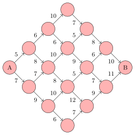
Consider the graph shown in Figure 17.4, where it is only possible to move to the right and the numbers associated with each edge represent a cost to traverse that edge. The decision to be made at each node is whether to go “up” or “down”, and we can assume the state transitions are deterministic.

diagram — Figure 17.4: Simple grid for shortest-path problem.

For this exercise:

1.

Use dynamic programming to find the shortest path from A to B.
2.

Consider a generalized version of the shortest path problem in Figure 17.4 where the grid has $n$ segments along each side. Find the number of computations required by an exhaustive search algorithm (i.e., the number of routes that such an algorithm would need to evaluate) and the number of computations required by a DP algorithm (i.e., the number of DP evaluations). For example, for the $n=3$ case shown in Figure 17.4, an exhaustive search algorithm requires 20 computations, while the DP algorithm requires only 15.

Problem 2: Machine Maintenance

Suppose we have a machine that is either running or is broken down. If it runs throughout one week, it makes a gross profit of $\$100$ . If it fails during the week, gross profit is zero. If it is running at the start of the week and we perform preventive maintenance, the probability that it will fail during the week is $0.4$ . If we do not perform maintenance, the probability of failure is $0.7$ . However, preventative maintenance will cost $\$20$ . When the machine is broken down at the start of the week, it may either be repaired at a cost of $\$40$ , in which case it will fail during the week with a probability of $0.4$ , or it may be replaced at a cost of $\$150$ by a new machine that is guaranteed to run through its first week of operation. Find the optimal repair, replacement, and maintenance policy that maximizes total profit over four weeks, assuming a new machine at the start of the first week (that is guaranteed to run during the first week of operation).

Problem 3: Markovian Drone

In this problem, we will model the task of flying a drone to its destination through a storm as a Markov Decision Process (MDP), and solve for the optimal policy using dynamic programming. The world is represented as an $n\times n$ grid, so the state space is:

\mathcal{X}\coloneqq\{(x_{1},x_{2})\in\mathbb{R}^{2}\mid x_{1},x_{2}\in\{0,1,% \dots,n-1\}\}.

In these coordinates, $(0,0)$ represents the bottom left corner of the map and $(n-1,n-1)$ represents the top right corner of the map. From any location $x=(x_{1},x_{2})\in\mathcal{X}$ , the drone has five possible controls it can apply:

\mathcal{U}\coloneqq\{\texttt{up},\texttt{down},\texttt{left},\texttt{right},% \texttt{land}\}.

The corresponding state changes for each control input are:

•

up: $(x_{1},x_{2})\mapsto(x_{1},x_{2}+1)$
•

down: $(x_{1},x_{2})\mapsto(x_{1},x_{2}-1)$
•

left: $(x_{1},x_{2})\mapsto(x_{1}-1,x_{2})$
•

right: $(x_{1},x_{2})\mapsto(x_{1}+1,x_{2})$
•

land: $(x_{1},x_{2})\mapsto(x_{1},x_{2})$

Additionally, there is a storm centered at $x_{\mathrm{eye}}\in\mathcal{X}$ . The storm’s influence is strongest at its center and decays farther from the center according to the equation $\omega(x)=\exp\left(-\frac{\lVert x-x_{\mathrm{eye}}\rVert_{2}^{2}}{2\sigma^{2% }}\right)$ . Given its current state $x$ and control input $u$ , the drone’s next state is determined as follows:

•

The control to land is deterministic.
•

With probability $\omega(x)$ , the storm will cause the drone to move in a uniformly random direction (for non-landing controls).
•

With probability $1-\omega(x)$ , the drone will move in the direction specified by the control (for non-landing controls).
•

If the resulting movement would cause the drone to leave $\mathcal{X}$ , then it will not move at all. For example, if the drone is on the right boundary of the map, then moving right will do nothing.

The quadrotor’s objective is to reach $x_{\mathrm{goal}}\in\mathcal{X}$ as quickly as possible, so the cost function is the indicator function $g_{t}(x_{t})=1-I_{x_{\mathrm{goal}}}(x_{t})$ . In other words, the drone will receive a cost of $1$ whenever it is not at $x_{\mathrm{goal}}\in\mathcal{X}$ , and a cost of $0$ at the goal. The drone has limited fuel capacity, so it must reach the goal in at most $T$ timesteps. If the drone is not at the goal at the end of the horizon, it will crash and we will incur a cost of $100$ to replace the drone, therefore $g_{T}(x_{T})=100(1-I_{x_{\mathrm{goal}}}(x_{T}))$ .

In the notebook ch17/exercises/markovian_drone.ipynb, complete the following exercises:

1.

Implement the functions of DroneMDP to compute the optimal cost-to-go values via dynamic programming (Algorithm 2) and extract the optimal policy using Equation 17.14.
2.

Given $T=100$ , $n=20$ , $\sigma=10$ , $x_{\mathrm{eye}}=(15,15)$ , and $x_{\mathrm{goal}}=(19,9)$ , compute and plot a heatmap of the optimal cost-to-go for $t=0$ over the grid $\mathcal{X}$ . Then, using the code provided, simulate the MDP with the optimal policy for $T=100$ time steps with the state initialized at $x=(0,19)$ .

Practice · 1 notebooks

Markovian Drone Open in Colab Source