Individual sensors come with hard-wired limitations in terms of range, field of view, and resolution or quantization.
On top of these design limits, performance often degrades under certain environmental conditions1717. Liggins II, Martin, Hall, David, Llinas, James. Handbook of multisensor data fusion: theory and practice. CRC press, 2017.
Thrun, S., Burgard, W., Fox, D. Probabilistic Robotics. MIT Press, 2005..
In practice, sensors also age and occasionally fail: calibration drifts, biases grow, and sometimes a device drops out altogether.
The aim of sensor fusion is to design robotic systems that remain robust to individual sensor weaknesses by combining multiple, often heterogeneous, sensors so that their information collectively reduces uncertainty in perception and localization tasks1818. Gustafsson, F. Statistical Sensor Fusion. Studentlitteratur, 2013.
Simon, D. Optimal State Estimation: Kalman, $H_ $, and Nonlinear Approaches. John Wiley & Sons, 2006..
Why fusion helps.
Three recurring patterns motivate sensor fusion in real systems:
-
1.
Complementarity: Different sensor modalities observe different aspects of the world, such as geometry or appearance, and combining them reduces ambiguity.
-
2.
Redundancy: Multiple sensors that observe the same latent quantity allow resilience to noise spikes and dropouts via consistency checks and cross-validation.
-
3.
Cooperation: Two weak cues can form a strong one when combined, such as monocular vision paired with an IMU to recover metric scale.
At a high level, sensor fusion treats each sensor output as a probabilistic observation of the underlying state and then combines those observations to obtain a posterior belief that is sharper and more reliable than any single source.
Example 15.0.1 (Perception for autonomous driving).
A self-driving car typically uses a combination of lidar and radar for distance sensing. Lidar provides high-resolution geometric structure at short to medium range, while radar is more robust at longer ranges and in adverse weather1919. Samuel Blackman, Robert Popoli. Design and Analysis of Modern Tracking Systems. Artech House, 1999.††margin: Radar is also generally more robust than lidar in fog, rain, or snow. . Cameras complement distance sensors: they provide high spatial density and rich appearance cues for object recognition and semantics, and they supply accurate bearing information to landmarks and obstacles.
Figure 15.1 illustrates the idea in 2D. Radar measurements often have strong longitudinal (range) accuracy but weaker lateral resolution; cameras, by contrast, deliver accurate lateral bearing but poor absolute depth. Fusing the two yields a positional estimate that is precise both longitudinally and laterally.
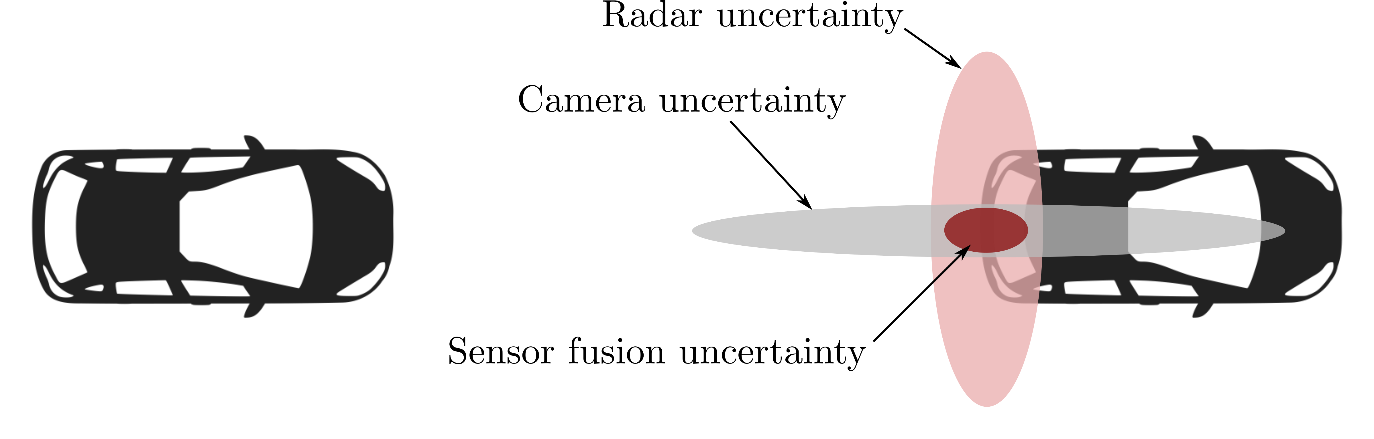
-1]Sensor fusion can reduce uncertainty by providing more well-rounded data. For example, a radar sensor may provide good longitudinal distance accuracy but slightly less lateral accuracy, and a camera may provide poor range estimation but good lateral position estimation. By fusing these two signals, the resulting position estimate can be accurate longitudinally and laterally.
Example 15.0.2 (Localization for ground robots).
A wheeled robot might use GNSS together with wheel encoders to estimate position. GNSS keeps global position error bounded, while encoders provide fine-grained, high-rate short-term motion increments. When GNSS is degraded or lost, such as in urban canyons or under foliage, encoder odometry can bridge the gap. Conversely, when wheel slip corrupts odometry, GNSS can pull drift back into line. As we will see, treating these sources probabilistically allows a filter to down-weight whichever one is less reliable at any moment.
Example 15.0.3 (Other common pairings).
Aerial robots often fuse a high-rate IMU with barometer and vision. The IMU stabilizes attitude and short-term motion, vision constrains drift and provides scale, and the barometer anchors altitude. Mobile manipulators combine joint encoders with depth sensing for precise end-effector placement while maintaining situational awareness. In all of these cases, no single sensor is sufficient across all operating regimes, but a carefully engineered combination is.
We will adopt a probabilistic perspective on fusion. Let denote the latent state and let be the set of measurements from all sensors. Under suitable assumptions, fusion is described by the posterior belief:
which we will realize with Kalman-family filters and their nonlinear and distributed variants. The same viewpoint also underpins modern learning-based systems, where we often fuse intermediate features rather than raw measurements.
In this chapter, we first introduce a taxonomy of fusion modes and architectures, then develop Bayesian fusion using linear and nonlinear filters, including bias-aware modeling and conservative strategies for unknown correlations. We discuss practical issues such as spatial registration, time alignment, multi-rate/asynchronous updates, and out-of-sequence measurements. We then connect fusion to object tracking, covering gating and data association (GNN/JPDA/MHT) as well as advanced random finite set (RFS) methods, and finally survey modern practice in feature- and BEV-level fusion, uncertainty calibration for learned modules, and cooperative (V2X) perception. Throughout, we tie the abstractions back to real robotic systems using examples like those above.
15.1 A Taxonomy of Sensor Fusion
We begin by situating sensor fusion along three complementary axes: one describes the data we receive from sensors, one characterizes the fusion problem, and one describes the system architecture. Thinking through all three lenses helps identify both an appropriate mathematical formulation and the right engineering design choices for a given application.
Data-related taxonomy.
Real sensors are imperfect in several simultaneous ways. Measurements are uncertain due to stochastic noise, biased because of drifts and miscalibrations, and coarse due to finite resolution or quantization2020. Liggins II, Martin, Hall, David, Llinas, James. Handbook of multisensor data fusion: theory and practice. CRC press, 2017.. Beyond these first-order issues, real systems often exhibit:
-
•
Correlations across streams, for example due to shared timing, mounting, vibrations, or processing pipelines.
-
•
Disparities between modalities, such as different range envelopes and failure modes.
-
•
Outright inconsistencies, such as outliers, contradictory readings, or disorder due to out-of-sequence arrivals.
Robust fusion methods must explicitly acknowledge these realities. In this chapter, we will model noise and bias (Section 15.2.1), guard against cross-stream double-counting when correlations are unknown (Section 15.2.2), and handle asynchrony and delayed packets with fixed-lag smoothing (Section 15.3.4).
Fusion-related taxonomy.
It is also useful to classify problems by what we fuse. At the lowest level, we combine raw or lightly processed time series such as range readings or pixel measurements. At an intermediate level, we fuse features or representations such as bird’s-eye-view (BEV) representations or learned embeddings. At a high level, we fuse decisions such as detections, tracks, or maps. These are often termed early, mid, and late fusion. All three appear in practice and impose different constraints on bandwidth, latency, and calibration.
Orthogonal to the representational choice is the relationship among sensors, leading to competitive fusion, complementary fusion, and cooperative fusion. In competitive fusion, redundant measurements of the same quantity are combined to improve reliability via consistency checks. In complementary fusion, we combine sensors that see different aspects of the world, such as lidar for short-range geometry and radar for long-range motion, to fill in gaps and reduce ambiguity. In cooperative fusion, sensors recover information that no single one can provide alone, as when monocular vision acquires metric scale only when paired with inertial sensing††margin: For example, GNSS localization and stereo vision can be cooperatively fused because they measure fundamentally different properties of the environment. .
In this chapter, we give each of these a probabilistic interpretation, treating every stream as a stochastic observation, and show how the choice of level and relationship guides the appropriate update rules and statistical tests (the referenced section).
Architectural taxonomy.
Finally, we classify fusion by where the computation takes place. In a centralized architecture, raw data or features are transported to a fusion center that estimates the state using all information at once. This is statistically efficient but demands bandwidth and creates single points of failure. In a decentralized architecture, each platform or subsystem runs a local estimator and transmits summaries, such as tracks with covariances, to a higher layer that fuses posterior distributions. This reduces raw bandwidth but raises questions about cross-correlation. In a distributed architecture, peers exchange beliefs or innovations over a communication graph and seek agreement via consensus or information sharing. Such architectures scale naturally to vehicle-to-everything (V2X) and multi-robot scenarios but must preserve consistency when cross-covariances are unknown. We will see how information-form filters support decentralized and distributed updates, and how conservative schemes such as Covariance Intersection maintain correctness in the face of unknown dependencies (Section 15.4)2121. Reza Olfati-Saber, J. Alex Fax, Richard M. Murray. “Consensus and Cooperation in Networked Multi-Agent Systems.” Proceedings of the IEEE 95(1), 215–233, 2007..
These three taxonomies—imperfections in the data, the level and relationship of fusion, and the architecture of computation—provide a scaffold for the remainder of the chapter. We move from Bayesian formulations and Kalman-family updates to the practicalities of registration and asynchrony, then on to multi-object tracking and modern feature/BEV-level fusion, referring back to this taxonomy to justify design choices along the way.
15.2 Bayesian Approach to Sensor Fusion
In previous chapters, we introduced Bayes-filter-based algorithms for state estimation and localization. The very same viewpoint naturally solves sensor fusion: each sensor contributes a probabilistic observation of the latent state, and Bayes’ rule combines these contributions into a posterior belief that is more precise and more reliable.
Beliefs, likelihoods, and Bayes’ rule.
We model unknown quantities as random variables and represent knowledge as probability distributions. Let denote the latent state at time and let be the set of measurements from sensors at that time. Under the assumption that the measurements are conditionally independent given , the Bayesian update from prior is:
| (15.1) |
If this conditional independence assumption does not hold, we must either model the joint likelihood (including cross-covariances) or use conservative fusion strategies that remain valid under unknown correlations (Section 15.2.2). In either case, the product of likelihoods in Equation 15.1 formalizes the intuition that multiple sensors together reduce uncertainty.
Why the Bayesian approach?
The Bayesian viewpoint is attractive for several reasons:
-
•
It provides a unified, interpretable representation of information: any modality that can be probabilistically modeled can be expressed as a likelihood over the state.
-
•
It natively handles uncertainty††margin: For example, the variance of a Gaussian posterior quantifies dispersion. Calibrated posteriors therefore allow principled gating and fault detection. .
-
•
It offers a principled update rule via Bayes’ theorem and naturally handles missing data, delayed packets, and novel observations.
Example 15.2.1 (Probabilistic competitive fusion).
Consider two sensors measuring the same scalar quantity , producing measurements and with Gaussian noise:
Treating the likelihood as a function of , their product is proportional to a Gaussian in :
The maximum-likelihood estimate of is therefore a precision-weighted average of and , and the joint uncertainty strictly decreases: .
If we also incorporate a Gaussian prior , the posterior remains Gaussian with:
and the earlier result is recovered in the uninformative-prior limit .
15.2.1 Linear-Gaussian Fusion: The Kalman Filter
The Kalman filter, introduced in Chapter 12, is the linear-Gaussian instance of the Bayesian filter and a workhorse for sensor fusion. We assume linear dynamics:
and a linear measurement model:
with a Gaussian belief . Here is the process-noise covariance and is the measurement-noise covariance, which may encode multiple sensors.
Prediction update.
The Kalman filter prediction step is:
where and denote the predicted mean and covariance at time .
Measurement update (stacked multi-sensor form).
Suppose sensors report at time . We stack their measurements into a single vector:
where and are the measurement matrix and noise covariance for the -th sensor. Then:
and the update becomes:
Sensors with smaller covariance in are automatically weighted more heavily in the Kalman gain††margin: This is visible in . .
Information form (useful for decentralized/distributed fusion).
Define the information matrix and vector by and . Each independent measurement block contributes:
Fusion then reduces to summation:
This additive structure makes it natural to combine multi-sensor updates or exchange increments over a network, as we will discuss in Section 15.4.
Innovation tests and gating.
Define the innovation and its covariance as above. The Normalized Innovation Squared (NIS):
follows a distribution of appropriate dimension under correct modeling. We will use this to gate outliers††margin: We revisit gating in Section 15.5.2. , detect faults, and monitor consistency.
Augmenting the state (bias-aware fusion).
A powerful trick is to augment the state with nuisance parameters such as sensor biases or calibration terms. For an additive bias , we define the augmented state:
and a measurement becomes linear in with measurement matrix . This allows the filter to learn biases online and prevents them from masquerading as state errors. Scale or misalignment biases can be handled similarly with appropriate parameterizations.
Nonlinear sensors: EKF and UKF.
For nonlinear measurements , we can either linearize via the Jacobian and apply the extended Kalman filter (EKF), or propagate sigma points through in the unscented Kalman filter (UKF). Both preserve the Bayesian structure, and the UKF generally performs better on strongly nonlinear problems. Bias augmentation and stacked updates carry over unchanged.
Example 15.2.2 (Kalman filter multi-sensor fusion).
Consider a self-driving car equipped with an IMU, a GNSS receiver, and a lidar sensor. We estimate longitudinal position , velocity , and acceleration using a constant-acceleration kinematic model:
Discretizing with sampling time and allowing process noise gives
Suppose lidar and GNSS measure the position , and the IMU measures the acceleration :
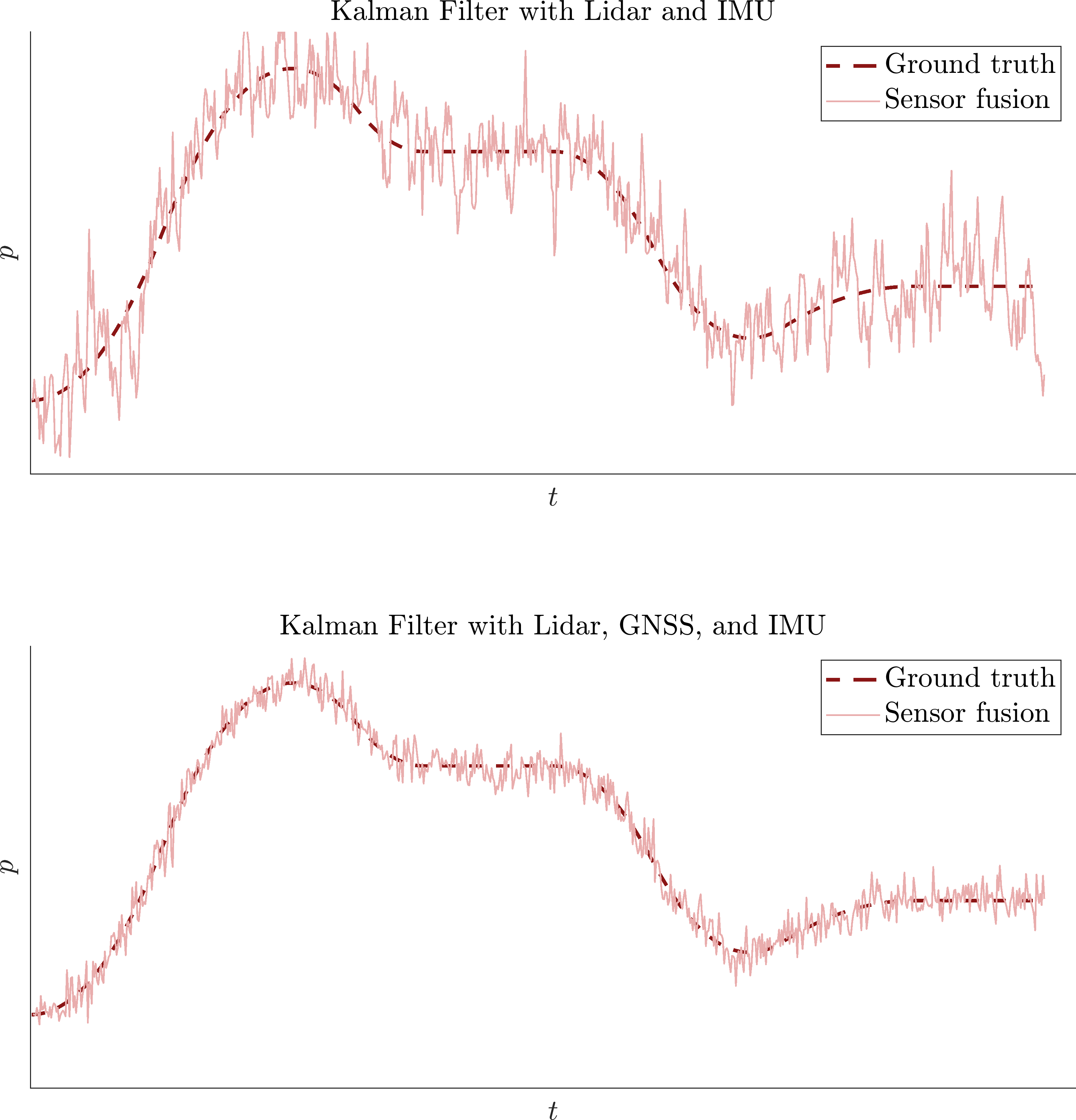
Here stacks the sensor variances, , , and . Figure 15.2 shows that adding a lower-variance GNSS channel tightens the position estimate and reduces noise††margin: Even a noisier additional sensor can help by improving observability or by providing redundancy for fault detection, but the effect is more modest. . The relative weighting is handled automatically by the Kalman gain.
15.2.2 Unknown Correlations and Conservative Fusion
When fusing estimates from separate filters††margin: For example, in track-to-track fusion, decentralized networks, or when reusing map priors. , cross-covariances are often unknown. Naively fusing them as if they are independent produces overconfident posteriors. A principled, conservative alternative is Covariance Intersection (CI), which combines Gaussian estimates without requiring cross-covariances. Given and , CI defines:
with chosen to minimize, for example, or . CI guarantees consistency irrespective of the true, unknown correlation structure and will reappear in our discussion of distributed fusion in Section 15.4.
In summary, the Bayesian lens turns the problem of sensor fusion into a precise algebra over beliefs and likelihoods. Linear-Gaussian assumptions yield closed-form Kalman filters with simple stacked updates and an additive information form, mild nonlinearities are handled by EKF/UKF variants, and practical wrinkles such as biases, asynchrony, and unknown correlations are addressed with state augmentation, smoothing, and conservative fusion. We build on this foundation in the next sections.
15.3 Engineering Realities: From Models to Working Systems
The Bayesian rules from the previous section tell us how to combine beliefs and likelihoods. Real robots, however, add a layer of practical complexity: sensors are mounted somewhere on the body and point in particular directions, they operate at different rates with different latencies, networks drop or reorder packets, and multiple streams may be subtly correlated. This section bridges the gap between the clean algebra of Bayes’ rule and systems that survive contact with hardware.
We move from where a sensor lives (spatial registration), to when it speaks (time alignment and multi-rate updates), to what happens when it speaks late (out-of-sequence measurements), and finally to staying honest about information (unknown correlations and faults).
15.3.1 Spatial Registration and Calibration
Before any fusion can succeed, measurements must be made commensurate with per-sensor intrinsics††margin: Such as a camera’s focal length and distortion, an IMU’s scale factors and axis misalignment, or a radar’s range/Doppler scaling. and extrinsics††margin: The rigid transform from each sensor frame to the body frame and, where needed, from the body to a global frame. . Calibration is not a one-time event: temperature changes, mechanical wear, and firmware updates can shift sensor parameters over time. A filter that appears increasingly overconfident often points to registration that has drifted out of spec.
A useful way to understand the effect of small miscalibration is to linearize it. If a measurement depends on the transform from body to sensor , denoted , through some function , then around a nominal we can write:
where is a small pose perturbation, is its sensitivity, and is sensor noise. This first-order view suggests two complementary strategies:
-
•
Treat extrinsics as known but uncertain: inflate the measurement covariance by , where encodes extrinsic uncertainty. This preserves consistency without changing the state.
-
•
Augment the state with a minimal parameterization of the extrinsic and assign it a slow random-walk prior. The filter then learns small misalignments online rather than forcing other states to absorb them.
Example 15.3.1 (Online camera–lidar extrinsics).
A mobile platform relies on a pre-calibrated extrinsic transform . Over weeks, thermal drift subtly increases the innovation statistics (NIS) of the camera measurements. By augmenting the filter state with a six-degree-of-freedom perturbation of and adding sparse visual–depth correspondences as pseudo-measurements, the system recenters the alignment online. A small process noise on the extrinsic states prevents overfitting transient effects.
15.3.2 Time Alignment, Latency, and Stamps vs. Arrival
Sensors almost never report in lockstep time. They are clocked by different oscillators, traverse different processing pipelines, and communicate through different buses. The filter, however, should apply each measurement at the time it was taken. Accurate measurement timestamps are therefore critical; arrival times are, at best, indirect clues.
Hardware triggers or disciplined clocks, such as those using Network Time Protocol (NTP) or Precision Time Protocol (PTP), reduce relative drift. Additionally, known fixed latencies, such as a camera’s ISP delay, should be subtracted so that time stamps reflect exposure times, not the end of the processing chain. When an update is due at an intermediate time between filter steps, the state should be interpolated to before applying the measurement. For inertial navigation, IMU data can be preintegrated over to produce a relative-motion pseudo-measurement consistent with geometry, removing the need to resample at the IMU rate.
Example 15.3.2 (Stamp vs. arrival time matters).
A radar packet arrives at s with a timestamp s. If the filter treats the packet as if it were taken at s, the update is effectively “time-shifted,” biasing the estimate and corrupting the covariance. Maintaining a short, time-ordered buffer of states and applying the update at avoids this problem and sets the stage for proper handling of genuinely late packets in Section 15.3.4.
15.3.3 Multi-Rate and Asynchronous Updates
On a typical platform, the IMU runs at hundreds of Hertz, cameras at a few tens, lidar somewhere in between, and GNSS in single digits. The Kalman family naturally accommodates this: we predict forward to the next measurement time, and we update whenever a packet arrives.
In software, it is convenient to maintain a priority queue keyed by measurement time. The filter repeatedly advances (predicts) to the earliest timestamp, next applies††margin: Stacking multiple measurements with the same stamp into a single block so that the innovation covariance reflects their joint effect. all measurements with that timestamp, and then repeats. This simple discipline—“predict to the stamp, then stack at the stamp”—prevents subtle double counting and preserves the meaning of NIS tests used later.
15.3.4 Out-of-Sequence Measurements and Fixed-Lag Smoothing
Even with careful time stamping, networks reorder and delay packets. A classical example is GNSS delivered over a congested channel, where a position measurement computed at time may arrive at time . Applying the measurement at the head of the filter timeline warps the uncertainty and can cause visible jumps in the estimate. The remedy is to keep a short history and re-solve the portion of the problem that lies within that window. A high level procedure for fixed-lag Rauch–Tung–Striebel (RTS)2222. Rauch, Herbert E, Tung, F, Striebel, Charlotte T. “Maximum likelihood estimates of linear dynamic systems.” AIAA journal 3(8), 1445–1450, 1965. smoothing for out-of-sequence measurements is:
-
1.
Fix a lag and maintain a buffer of estimates together with the dynamics . Suppose a measurement with arrives.
-
2.
Run an RTS backward pass from back to to compute smoothed estimates (and, if needed, cross-covariances).
-
3.
Insert the update at using as the prior.
-
4.
Re-propagate forward from to , re-applying any later measurements in the buffer.
-
5.
Commit the corrected states.
The lag should exceed typical delay jitter. If a packet falls outside the window, we can either discard it or assimilate it approximately with an inflated, time-shifted update.
Example 15.3.3 (GNSS delay in a lidar–IMU EKF).
An EKF runs at IMU rate ( Hz) with lidar odometry updates at Hz. GNSS packets occasionally arrive ms late. With a fixed lag s, the filter back-smooths, inserts the GNSS update at its true time, and re-propagates. The NIS distribution tightens, and the trajectory becomes free of the jumps that were present when late packets were applied at the head of the queue.
15.3.5 Unknown Correlations, Double Counting, and Consistency
Fusion is not only about more data, it is about honest information. Measurement streams may be correlated because they share process noise††margin: For example, the sensors are mounted on the same body. , because they reuse the same map or prior, or because one stream already incorporates measurements from the other. If cross-covariances are known, they can be modeled explicitly. Often they are not, and fusing as if streams were independent yields overconfident covariances: NIS and NEES statistics will then fail checks.
Several responses are available:
-
•
When possible, exchange innovations (residuals and their covariances) rather than full posteriors, since innovations are closer to independent across nodes.
-
•
When that is insufficient, conservative fusion methods such as Covariance Intersection (Section 15.2.2) combine Gaussians without any knowledge of cross-covariances and guarantee consistency at the price of modest optimality.
-
•
In all cases, monitor empirical NIS/NEES against theoretical quantiles and treat persistent deviations as feedback that some correlation, timing error, or noise model has been overlooked.
15.3.6 Fault Detection and Isolation
Even a well-registered, well-timed system must protect itself against bad data. Kalman filters already provide a convenient diagnostic: the innovation and its covariance define the NIS , which under a correct model follows a distribution of known dimension. Setting a gate at a chosen significance level rejects gross outliers, and tracking moving averages of the NIS per sensor exposes slow degradation.
When a sensor begins to misbehave, there are two complementary reactions:
-
•
Innovation-based adaptive estimation: inflate that sensor’s measurement covariance according to a feedback law derived from recent NIS so that the filter automatically down-weights it.
-
•
Structural response: if the issue resembles a bias or scale error more than random noise, augment the state with the offending parameter and let the filter learn it.
In systems with redundancy††margin: Two or more sensors nominally measuring the same quantity. , it is natural to maintain a per-sensor health score and to prefer the healthier stream while keeping the others alive for fault detection and graceful recovery.
Example 15.3.4 (Rain on a camera, radar nominal).
During a storm, the camera’s measurements intermittently fail the NIS gate, while radar remains nominal. The system inflates the camera’s measurement covariance and leans more heavily on radar for range and velocity. Once the rain clears and the camera’s NIS returns to expected quantiles, its weight rises automatically. Throughout, the reported covariance remains conservative, so downstream planners are not surprised.
15.3.7 Numerical Stability and Practical Monitors
A few numerical practices are particularly useful. First is the use of square-root filters, which propagate a Cholesky factor of to be more stable than propagating directly, and help prevent negative-definite covariances due to round-off. Second, when updating the covariance we can use the Joseph stabilized form:
which preserves positive semidefiniteness in finite precision. On the monitoring side, plotting NIS/NEES histograms with overlays, tracking the determinant and condition number of , and logging gate hit-rates and stamp-minus-arrival statistics provide early warnings for timing and calibration regressions.
Takeaway.
Registration and timing turn raw measurements into commensurate evidence; buffering and smoothing reconcile the past with the present; and attention to correlation and faults keeps the estimator honest. With these pieces in place, we can extend from single-state fusion to the challenges of object tracking and the demands of distributed systems, which we address next.
15.4 Fusion Architectures
The Bayesian viewpoint tells us how evidence should be combined and the architecture decides where the combination happens and what is exchanged. In practice, three recurring patterns emerge: centralized systems that gather everything in one place, decentralized systems that fuse local tracks at a higher layer, and distributed systems that reach agreement over a network. Each involves trade-offs in bandwidth, latency, robustness, and the ease of maintaining consistent uncertainty (Section 15.3.5).
15.4.1 Centralized Fusion
Centralized designs are conceptually simplest: raw measurements or lightly processed features are transported to a single estimator that maintains the posterior over the state. Mathematically, this is just the stacked update in Section 15.2.1, where at time we form:
compute the innovation and its covariance , and apply a single Kalman update. Centralized fusion is statistically efficient and gives the clearest path to proper gating, bias handling, and OOSM smoothing (the referenced section).
Its limitations are operational rather than mathematical. Communicating raw sensor streams consumes bandwidth, creates central bottlenecks and single points of failure, and can be awkward when sensors live on different platforms, such as across vehicles and infrastructure. A common compromise is to centralize only within a platform or robot, fusing camera/lidar/radar/IMU locally and exposing higher-level artifacts—detections, tracks, occupancy—to the outside world.
15.4.2 Decentralized Track-to-Track Fusion
In a decentralized system, each subsystem or platform runs its own filter and publishes summarized beliefs—typically a state estimate with covariance and, possibly, a timestamp and a health score. A fusion node then combines these “tracks”2323. Zhang, Shuo, Bar-Shalom, Yaakov, Watson, Gregory. “Tracking with multisensor out-of-sequence measurements with residual biases.” In 2010 13th International Conference on Information Fusion, 1–8, 2010.. The main question is how to fuse them without breaking consistency.
If the contributing tracks are conditionally independent given the true state††margin: For example, if they use disjoint raw measurements. , fusion is straightforward in information form. If a local node transforms a common prior into , it can transmit its increment:
and the fusion node simply adds the increments from all sources:
In the linear-Gaussian case, these increments equal and for that node’s local measurements. This “common-prior + increment” view keeps the algebra exact, but it requires that all nodes agree on (or communicate) the prior against which those increments were formed.
When two tracks are not independent—because they share process noise, maps, or each other’s measurements—their cross-covariance is generally unknown. Fusing as if independent is then dangerous (Section 15.3.5). A safe default is Covariance Intersection (Section 15.2.2), which guarantees consistency at the cost of some conservatism2424. Julier, Simon J, Uhlmann, Jeffrey K. “A non-divergent estimation algorithm in the presence of unknown correlations.” In Proceedings of the 1997 American Control Conference (Cat. No. 97CH36041), 2369–2373, 1997.. If cross-covariances are known††margin: For example, in a carefully engineered multi-radar system with a common process model. , we can compute the optimal best linear unbiased estimator (BLUE) weights using the joint covariance of the two track estimates. In practice, the engineering overhead to maintain those cross-terms often outweighs the marginal gain over CI.
Example 15.4.1 (Track-to-track fusion with equivalent information).
Two drones estimate a shared target’s position. Each runs a local EKF and, at each second, exports the pair computed from its local pre- and post-update information states. A ground station maintains a common prior and updates it by addition. Because increments are additive and tied to a common prior, the result matches exactly what would have been obtained had the ground station received both raw measurement streams centrally. If a communications hiccup delays one drone’s packet, the ground station treats it as an out-of-sequence increment and inserts it using the same fixed-lag machinery as in Section 15.3.4.
15.4.3 Distributed Fusion by Consensus and Information Exchange
Truly distributed systems have no fusion center. Instead, peers exchange messages over a communication graph and attempt to agree on the posterior. The information form makes this natural: at each time step, node computes its local increment from its own measurements, then the network mixes these contributions so that everyone converges to the same sum.
One simple version is average consensus on information increments using a symmetric, doubly stochastic mixing matrix that respects the communication graph. Assume all nodes start from the same prior . Each node initializes its local consensus state from its own increment:
Then perform rounds of neighbor averaging:
When the graph is connected and is well chosen, and converge to the network-wide averages of the increments. An exact centralized posterior is then recovered by multiplying by the number of nodes :
In directed or time-varying graphs, push-sum or diffusion variants play the same role. In practice, a small number of rounds††margin: Even or . often captures most of the benefit.
Correlation again requires care. If nodes are connected through shared process models or re-used features, repeated neighbor mixing can re-inject the same evidence multiple times. Two mitigations are common. First, we can exchange innovations rather than full posteriors, since these tend to be closer to independent across nodes. Second, we can replace consensus averaging with CI-consensus: combining neighbors’ information conservatively when independence is doubtful so each node’s covariance remains an upper bound on its true error.
15.4.4 What to Send: Raw Data, Features, or Tracks?
Architectures are inseparable from communication budgets. A useful mental model is to choose a bandwidth tier:
-
•
Raw or ROI data††margin: For example, point clouds or image crops. : maximal accuracy and flexibility, but highest bandwidth, strict latency requirements, and potential privacy concerns.
-
•
Features or bird’s-eye-view (BEV) grids: a strong trade-off in modern stacks; semantics are preserved, bandwidth is moderate, and time alignment can be handled at the feature level.
-
•
Decisions (detections, tracks, occupancy): minimal bandwidth and simplest to distribute; best suited to decentralized and distributed fusion, but with the least flexibility for correcting upstream errors.
Two additional practicalities:
-
•
Messages should carry uncertainty (covariances or credible intervals), not just point estimates, to enable principled fusion at the receiver.
-
•
Timing matters as much as content: include measurement timestamps, not just send times, so that receivers can place information correctly on their own timelines (the referenced section).
Example 15.4.2 (Cooperative perception at an intersection).
Consider an urban intersection with an instrumented roadside unit (RSU) and vehicles approaching from multiple directions. Each vehicle maintains a centralized, on-board fusion stack (camera/lidar/radar/IMU) and publishes a stream of tracks with covariances. The RSU runs its own perception stack from elevated cameras and a 4D imaging radar. A decentralized fusion server aggregates vehicle and RSU tracks via equivalent information increments tied to a common prior at Hz. Vehicles subscribe to this fused track set.
When bandwidth is plentiful, the RSU also publishes mid-level BEV features for regions of interest such as crosswalks. Nearby vehicles that can spare compute perform a short, two-round consensus step (Algorithm 1) on the BEV-derived information, which sharpens occupancy in occluded regions. During peak congestion, the system falls back to track-level CI fusion to preserve consistency under stronger correlations. The result is a layered architecture: centralized fusion within each agent, decentralized fusion at the server for robustness, and briefly distributed fusion among peers when conditions allow.
Takeaway.
Centralized fusion is the gold standard when bandwidth and compute permit it. Decentralized fusion scales well and is straightforward when independence holds (or CI is used when it does not). Distributed fusion achieves resilience and coverage across a network, provided that messages preserve timing, carry uncertainty, and respect the difference between independence and correlation. We now turn from what and where to fuse to the closely related problem of tracking multiple objects through time.
15.5 Object Tracking
Sensor fusion becomes especially important when the goal is not just an ego state but a changing population of objects: vehicles, pedestrians, drones, or landmarks that appear, move, occlude one another, and disappear. The task of object tracking is to estimate, through time, both the continuous states, such as positions and velocities, and the discrete identities of these objects given noisy, partial, and sometimes contradictory measurements.
In this section, we build a practical tracker from motion and measurement models, add principled gating to keep outliers at bay, address data association to decide which detection belongs to which track, and define track management to handle births, deaths, and occlusions. We close with an advanced view based on random finite sets and a brief tour of tracking-by-detection systems and evaluation metrics.
15.5.1 States, Motion Models, and Measurements
We model each target at time with a state vector and a measurement model that connects states to observed quantities. A common starting point for ground vehicles is a constant-velocity (CV) model in the plane:
with white-acceleration process noise:
For targets that turn, a coordinated-turn (CT) model augments the state with a turn rate and typically uses an EKF or UKF update. A constant-acceleration (CA) model can be more appropriate for pedestrians or stop-and-go traffic. The choice of model trades fidelity for simplicity; a good practice is to begin with CV and only move to CT or CA if innovation statistics suggest a benefit.
Measurements take many forms. A radar may report range , bearing , and sometimes radial velocity :
Camera detections may provide image-space bounding boxes and, if depth is available, 3D centroids in the ego frame. Lidar clusters similarly yield centroids and sometimes yaw estimates. We fold these into linear or linearized measurement models and apply the Kalman-family update from Section 15.2.1 for each track.
15.5.2 Gating and the Role of the Innovation
Before tackling the combinatorics of association, we narrow the search space with gating. Given a predicted measurement for a track and its innovation covariance , a detection is deemed compatible if the (squared) Mahalanobis distance:
lies below a threshold from the distribution at a chosen confidence††margin: For example, for a conservative, wide gate. . This is exactly the NIS concept from Section 15.3; under the model, follows for measurement dimension .
Gating dramatically reduces the clutter presented to the assignment solver: it retains almost all true matches while excluding most spurious ones.
Example 15.5.1 (Ellipsoidal gates in practice).
With radar range–bearing measurements (), a threshold near carves out an ellipse in measurement space. In dense traffic, this can reduce candidates per track from dozens to a handful, turning an intractable assignment into a manageable one while preserving nearly all true associations.
15.5.3 Data Association: From Nearest Neighbor to Probabilistic
After gating, we must decide which detection updates which track. The simplest approach is Global Nearest Neighbor (GNN): we define a cost matrix between track and detection (often using Mahalanobis distance), and solve the 2-D assignment problem with the Hungarian algorithm. Algorithm 2 summarizes a standard gated GNN pipeline with gating and occlusion handling. Unassigned tracks receive missed-detection events; unassigned detections may seed new tracks.
GNN is fast and effective in relatively unambiguous scenes, but it commits to a single hypothesis even when multiple associations are plausible. Two families of methods hedge this ambiguity.
Probabilistic (joint) data association (PDA/JPDA).
In Probabilistic Data Association (PDA), each track considers all detections in its gate and performs a mixture update weighted by association probabilities and a missed-detection probability . Joint PDA (JPDA) generalizes this to multiple tracks, computing a consistent set of probabilities across the scene.
For a track with prior and each candidate detection , we compute the innovation , its likelihood:
and then normalize (with clutter intensity included) to obtain the . For each candidate association , let denote the conditional KF/EKF posterior, and let denote the missed-detection case. JPDA then matches the first two moments of this mixture:
The second term inside the brackets captures residual association ambiguity, such that even if each conditional posterior is sharp, disagreement among the candidate means keeps the final covariance honest. JPDA’s main cost is combinatorial in the worst case, but clustering or pruning unlikely joint events keeps it tractable.
Multiple-hypothesis tracking (MHT).
Multiple-hypothesis tracking maintains a small forest of competing association histories and prunes them by likelihood. Each hypothesis carries its own set of track states. When new detections arrive, the tree branches over plausible assignments; pruning and N-scan backtracking keep the tree shallow. Deferred decisions across a short horizon can significantly improve performance in crowded, ambiguous scenes.
Appearance and motion together.
Motion models constrain where a target could go; learned appearance cues, such as embeddings from image crops or lidar shape descriptors, constrain who it likely is. A common composite cost is:
where is a detection embedding and is a track’s appearance model. Appearance reduces identity switches during occlusions and interactions, particularly in camera-heavy setups.
Example 15.5.2 (Ambiguity at a pedestrian crossing).
Two pedestrians cross paths inside each other’s gates. GNN alone risks swapping identities, but JPDA softens the update for both tracks across the ambiguous frames, while a modest appearance term, such as a color/texture embedding, stabilizes the assignment and preserves identities.
15.5.4 Track Management: Birth, Death, and Occlusion
Bookkeeping is a critical function for tracking modules. Good track management balances eagerness to explain new detections with skepticism that avoids proliferating false tracks.
Initiation.
Common strategies to initialize tracks include: M/N logic, which confirms a track only after hits in the last frames, and a score that accumulates matched updates and decays on misses. Initial covariances should be broad enough to reflect detector uncertainty and any depth ambiguity.
Maintenance and missed detections.
When a track receives no compatible detection, propagate its state through the motion model, inflate its covariance, and reduce its survival score. During short occlusions, this “coast” allows re-acquisition without identity breaks. Keep occluded tracks alive for at most seconds or frames, tunable to the scene.
Termination and hygiene.
Delete tracks that fail confirmation or whose survival score falls below threshold. Merge or split tracks when they overlap persistently or when one detection consistently explains two weak tracks better than the reverse. Periodically purge stale hypotheses in MHT and stale appearance embeddings.
15.5.5 Random Finite Set (RFS) Filters
When the number of targets varies and clutter is heavy, it is natural to treat the set of objects as the fundamental random variable. RFS filters propagate distributions over sets rather than over a fixed list of tracks.
PHD and GM-PHD.
The Probability Hypothesis Density (PHD) filter evolves the first moment (intensity) of the target-set distribution, whose peaks correspond to likely targets. With linear-Gaussian models, the Gaussian-mixture PHD (GM-PHD) filter maintains a set of weighted Gaussians with birth and survival terms. This approach is efficient, handles births and deaths gracefully, and works well when targets are numerous but relatively weak, though it does not manage identity explicitly.
Labeled multi-Bernoulli and -GLMB.
For identity-aware tracking, labeled multi-Bernoulli (LMB) and -GLMB filters maintain labeled tracks with existence probabilities. They offer principled handling of associations, births, and deaths within a Bayesian set framework. The cost is increased computation and bookkeeping, but in return they handle combinatorial association in a coherent manner and provide clean uncertainty accounting in heavy clutter.
RFS methods are not always necessary, but they are useful when scenes are dense, clutter rates are high, and identity is secondary to coverage (PHD) or when a full Bayesian treatment of multi-target tracking with identities (-GLMB/LMB) is desired.
15.5.6 Tracking-by-Detection and Modern Practice
Modern trackers often follow a tracking-by-detection paradigm, where a perception module (classical or learned) produces frame-wise detections with uncertainties, a motion model predicts track states, and an association layer links detections to tracks. In camera-centric systems, learned appearance embeddings significantly improve identity stability. In lidar/radar-centric systems, motion and geometry dominate, and appearance plays a smaller role.
Two themes recur:
-
1.
Uncertainty matters. Downstream gating and data association work much better when the detector exports calibrated confidence and geometric covariance (or a proxy such as a covariance in BEV cells). Calibrate these heads before fusion, for example with temperature scaling for classification and reliability diagrams for regression.
-
2.
Robustness to missing modalities. In adverse weather or partial failures, radar or thermal imaging may carry the burden. Design the tracker to operate with a subset of sensors by inflating the covariance of the missing modality, adjusting initiation thresholds, and tuning accordingly.
15.5.7 Evaluation: Metrics and What They Mean
Tracking quality is multi-faceted: we care about detection quality, geometric accuracy, and identity preservation. Three widely used metrics capture different aspects:
MOTA/MOTP.
Multiple Object Tracking Accuracy (MOTA) aggregates missed detections (FN), false positives (FP), and identity switches (IDSW) against the number of ground-truth objects (GT):
Multiple Object Tracking Precision (MOTP) summarizes localization error for correctly matched pairs. MOTA is simple and interpretable, but it can obscure trade-offs between detection and identity.
IDF1.
The IDF1 metric measures the F1 score of correctly identified detections over all matches, focusing on identity preservation. It penalizes identity swaps more explicitly than MOTA and is useful when appearance cues play a central role.
HOTA.
Higher Order Tracking Accuracy (HOTA) balances localization, detection, and association in a unified measure by scoring matched pairs over a range of thresholds and combining the resulting detection and association accuracies. It correlates better with human judgment in crowded scenes where identity stability matters.
A mature evaluation typically reports at least one association-aware metric (IDF1 or HOTA) alongside MOTA/MOTP and includes qualitative sequences that reveal behavior under occlusion, crossing, and sensor degradation. For safety-critical systems, also monitor calibration: plot innovation/NIS statistics for associated pairs to ensure the tracker remains consistent across conditions.
Takeaway.
A reliable tracker is not a single algorithm but a disciplined combination of realistic motion models, measurements with honest uncertainties, ellipsoidal gating to filter clutter, association that respects ambiguity (using appearance where it helps), and careful track management. In dense or high-clutter regimes, RFS methods provide a principled alternative that scales gracefully. With these pieces in place, we return to the broader fusion story in the learning era—feature-level fusion in BEV, cooperative perception, and uncertainty calibration—which shape where we fuse in modern stacks.
15.6 Learning-Era Fusion: Features, BEV, and Cooperation
The probabilistic view from earlier sections remains the backbone of modern perception, but practice has shifted in two important ways. First, many systems now fuse features rather than raw measurements, often in a shared bird’s-eye view (BEV) representation that aligns modalities in space and time. Second, the locus of fusion has moved beyond a single box: vehicles and infrastructure exchange information, and filters increasingly sit downstream of learned modules whose outputs carry (or should carry) uncertainty. This section turns these trends into concrete design patterns.
15.6.1 Where to Fuse: Early, Mid, or Late?
Classical fusion, as in Section 15.2.1, stacked raw measurements and operated directly on likelihoods. This remains the gold standard when bandwidth is ample and calibration is impeccable. Modern stacks, however, often benefit from two additional levels that better reflect computational and communication realities.
Early fusion (raw space).
Here we project measurements into a common geometric frame and combine them there. For example, we may project lidar points colored by camera radiance, radar range–Doppler points registered in the ego frame, and stereo depth “lifted” into 3D. The reward is geometric precision and simple physics-based likelihoods. The cost is high bandwidth, strict time alignment, and sensitivity to small calibration errors: a milliradian of extrinsic yaw drift that is barely noticeable in an image can become a meter of error at long range when projected onto the ground.
Mid-level fusion (feature space).
In mid-level fusion, each sensor produces features via a learned backbone, and those features are then fused in a representation designed for downstream tasks. BEV has become the workhorse: by lifting multiple camera views, lidar, and radar into a ground-aligned grid, we obtain a scene description that is geometry-aware, compact, and well matched to detection, tracking, and planning. BEV removes ego-motion, naturally accommodates occupancy and flow estimates, and plays well with both filters and learned modules.
Late fusion (decision space).
At the other end of the spectrum we fuse decisions: detections, tracks, or occupancy tiles with associated uncertainties. Late fusion is bandwidth-efficient and maps neatly onto decentralized and distributed architectures (Section 15.4). The trade-off is reduced flexibility: once an upstream detector has committed to boxes or tracks, there are fewer opportunities to correct miscalibration or recover missed evidence.
No single level is universally best. A pragmatic recipe is:
-
1.
Centralize within a platform at mid-level (BEV), where most accuracy-per-byte gains lie.
-
2.
Export late-level artifacts for cooperation across platforms.
-
3.
Maintain an early-level path only where the safety case demands it††margin: For example, an emergency braking stack that reads raw radar. .
15.6.2 BEV and Transformer-Style Fusion
The BEV idea is conceptually simple but rich in practice. We represent the local scene as a grid aligned with the ground plane and ego pose, and let each modality contribute to that grid in the way most natural for it. The payoff is a shared canvas on which geometry, semantics, and motion can be reasoned about jointly.
From cameras to BEV.
Multi-view image features extracted by a backbone are lifted into BEV either through explicit geometry, such as projecting along estimated depth, or attention mechanisms that aggregate image features at positions consistent with BEV queries. In the geometric case, a pixel with depth back-projects to the camera frame and then to the ego frame:
In the attention-based case, a BEV query at ground point gathers evidence across cameras with weights that depend on viewing geometry and learned compatibility, sidestepping brittle monocular depth estimates.
Lidar and radar to BEV.
Lidar contributes 3D points whose heights and intensities can be pooled (min/max/mean, or learned pooling) into BEV features. Radar adds range–Doppler–angle evidence highlighting long-range velocities and all-weather robustness. After alignment, the result is a multi-modal BEV tensor in which nearby cells carry detailed geometry and far cells carry coarser, velocity-centered context.
Temporal fusion.
Scenes evolve and sensors report at different times. BEV benefits from temporal memory in two complementary forms:
-
•
Geometric memory: warp the previous BEV by the ego motion between frames and aggregate it with the current BEV. This acts as a skip connection that respects kinematics.
-
•
Learned memory: apply spatiotemporal attention over a short buffer of BEV frames so the model can “remember” moving actors.
Both require ego motion used for alignment to be time-consistent with feature timestamps (Section 15.3.2). Otherwise, the network ends up compensating for misalignment rather than modeling the scene.
Outputs and uncertainty.
Heads attached to the multi-modal BEV tensor predict detections, occupancy, flow, and other downstream quantities. To keep fusion principled, these heads should emit calibrated confidences and, when possible, geometric covariances or credible intervals for positions and extents (Section 15.6.6). These outputs feed directly into gating and association (the referenced section) and determine how heavily a filter should trust each piece of evidence.
15.6.3 From Features to Filters: The Adaptor Pattern
Learned modules speak in logits, heatmaps, and BEV tensors; filters expect pseudo-measurements with covariances. An adaptor translates between these languages so that the Bayesian machinery from earlier sections can operate on learned outputs without any sleight of hand.
At its simplest, an adaptor takes a detection —a position, a covariance proxy, and a confidence—and turns it into a measurement with covariance suitable for a KF/EKF update. Algorithm 3 shows a simple per-detection adaptor. The crucial step is calibration: mapping to a covariance whose empirical NIS statistics match quantiles on held-out data. Once calibrated, learned detections and classical sensors inhabit the same probabilistic currency.
Example 15.6.1.
A BEV detector yields a 3D position estimate and a covariance proxy from a covariance head. We define and update a platform-centric track with and , where is learned or fitted offline so that the NIS aligns with on validation sequences. The update then proceeds identically to a classical sensor, including gating and fault handling.
15.6.4 Cooperative Perception (V2X)
A single vehicle’s field of view is limited by its own geometry and occluders such as other vehicles and buildings. By contrast, an intersection camera may “see around corners,” and neighboring vehicles can reveal what an ego vehicle cannot. Cooperative perception asks three questions: what should we send, when should we send it, and how should the receiver fuse it while maintaining honest uncertainty?
What to send.
The tiers from Section 15.4.4 apply directly. Raw or ROI snippets are rich but expensive, mid-level BEV tiles carry useful context at manageable bitrate, and late-level tracks and occupancy are lightweight and easy to fuse. In practice, a layered strategy often works best: share BEV features for critical regions, such as blind corners, and share tracks elsewhere.
When and how.
Messages must carry measurement timestamps so receivers can place them correctly in their own timelines (Section 15.3.2). Relative pose between agents should be maintained by a small filter on with an associated covariance. That pose uncertainty should then propagate either into feature alignment (wider attention kernels, conservative warps) or into track fusion weights. Fusing as if poses were perfect is a quick way to become overconfident.
Fusion modes.
Feature-level cooperation aligns and aggregates BEV tiles—often with a learned attention block that explicitly accounts for pose uncertainty. Track-level cooperation uses the decentralized and distributed methods of Section 15.4; when independence is doubtful, Covariance Intersection (Section 15.2.2) provides a conservative backstop that preserves consistency.
Example 15.6.2 (Occlusion busting at a four-way stop).
A vehicle approaches a four-way stop occluded by a truck. The roadside unit (RSU) shares a narrow strip of BEV features covering the blind zone at Hz. The vehicle fuses these with its own BEV via attention, then initializes two pedestrian tracks with calibrated covariance. A neighboring vehicle’s track messages arrive a moment later; CI fuses them conservatively with the ego tracks, shrinking uncertainty without overstating confidence. The planner receives a consistent occupancy map and honest covariances.
15.6.5 Differentiable Filtering and Hybrid Models
Filters and networks are complementary rather than competing tools. Three hybrid patterns recur in modern systems.
Learned dynamics residuals.
We retain a physically grounded motion model (CV/CT) but allow a network to predict a residual acceleration or steering term from context (maps, intents, social cues). The filter then predicts with the combination of physics and learned residual, and the residual’s variance reflects confidence in the learned component. This improves short-term forecasting without abandoning structure.
Learned measurement models.
Instead of hand-coding the measurement model , we can learn a mapping from features to pseudo-measurements with a covariance head. The adaptor in Section 15.6.3 ensures that outputs are calibrated before they reach the filter, keeping NIS/NEES in check.
Back-propagating through filters.
For end-to-end tuning, we can unroll a few filter steps and back-propagate through the Kalman updates to adjust the feeding network. However, some safeguards are important: keep gains and covariances positive definite, regularize to avoid collapsing uncertainty, and validate with held-out NIS/NEES so the filter remains a filter rather than a brittle function approximator.
15.6.6 Uncertainty You Can Trust
Neural modules are powerful, but their confidence estimates are often miscalibrated, and fusion depends on honest uncertainty to avoid gates admitting outliers and associations overcommitting. Three classes of tools help keep confidence in line with reality: calibration, deep ensembles (or evidential models), and conformal prediction.
Calibration (post-hoc).
For classification, temperature scaling rescales logits by a scalar , chosen on a validation set, before applying softmax, improving calibration2525. Guo, Chuan, Pleiss, Geoff, Sun, Yu, Weinberger, Kilian Q. “On calibration of modern neural networks.” In International conference on machine learning, 1321–1330, 2017.. For regression, we can fit an affine map from raw variance proxies to empirical errors so predicted variances match residuals. Expected calibration error (ECE) and reliability diagrams provide simple diagnostics and can be tracked across conditions.
Deep ensembles and evidential models.
Small ensembles††margin: For example, three to five seeds. average predictions and expose epistemic uncertainty via disagreement2626. Lakshminarayanan, Balaji, Pritzel, Alexander, Blundell, Charles. “Simple and scalable predictive uncertainty estimation using deep ensembles.” Advances in neural information processing systems 30, 2017.. Evidential models predict parameters of a distribution over distributions††margin: For example, a Normal–Inverse-Gamma for scalar regression. , so uncertainty grows in regions with limited training data2727. Amini, Alexander, Schwarting, Wilko, Soleimany, Ava, Rus, Daniela. “Deep evidential regression.” Advances in neural information processing systems 33, 14927–14937, 2020.. Either way, we feed the resulting variance through the adaptor so that gates and gains respond quantitatively.
Conformal prediction for finite-sample guarantees.
Conformal methods wrap any base predictor and produce prediction sets with coverage without distributional assumptions2828. Angelopoulos, Anastasios N, Bates, Stephen et al. “Conformal prediction: A gentle introduction.” Foundations and trends in machine learning 16(4), 494–591, 2023.. For detections, a simple nonconformity score is negative log-likelihood or with ground truth on a calibration set. Given a quantile of scores, at test time we:
-
•
accept only predictions with score , or
-
•
inflate their covariance until the score would fall below .
This yields explicit, finite-sample control of false exclusion at the level of detections flowing into the tracker and keeps downstream gating behavior predictable.
15.6.7 Asynchrony, Events, and Adverse Weather
Two additional practical issues round out the learning-era picture.
Event cameras and asynchrony.
Event sensors report brightness changes at microsecond latency with large dynamic range. They pair naturally with IMUs and frame cameras: the IMU stabilizes short-term motion, event sensors add blur-free edges, and frame cameras add texture. Fusion follows the same timing discipline as in Section 15.3.2: respect timestamps, interpolate priors, and back-smooth when out-of-sequence events matter.
All-weather complements.
Rain, fog, and snow degrade cameras and lidar before radar and thermal imagers fail. Radar and thermal should therefore be treated as complementary modalities, not afterthoughts. During training, modality dropout in BEV fusion helps the network succeed when one input is missing. Online, the system inflates the covariance of degraded modalities and uses health scores (Section 15.3.6) to adapt sensor weights. The goal is graceful degradation: performance should bend under adverse conditions but not break.
Takeaway.
Learning-era fusion does not replace the Bayesian core; it builds on it. BEV provides a geometry-aware workspace where heterogeneous features meet, cooperative perception broadens the field of view, hybrid models let learning fill in what physics leaves out, and calibration and conformal wrappers keep uncertainty honest.
15.7 Summary
Sensor fusion is not a single algorithm but a way of organizing information. We began with a probabilistic lens: sensors provide likelihoods over latent quantities, and Bayes’ rule combines them into a posterior (Section 15.2). Under linear–Gaussian assumptions this reduces to the Kalman filter with stacked multi-sensor updates and an additive information form; with mild nonlinearities, we can extend to EKF/UKF. Along the way we introduced practical methods: augmenting states to absorb biases, gating with innovation tests to keep outliers from steering the estimate, and—when fusing external estimates—preferring conservative schemes such as Covariance Intersection over fragile independence assumptions.
To implement fusion in practice, we saw the importance of respecting the timing of measurements. Registration aligns frames so measurements are commensurate; timing discipline ensures updates occur at the measurement timestamp, not arrival time; multi-rate and asynchronous updates are handled by “predicting to the stamp, then stacking at the stamp”; and late packets are reconciled by fixed-lag smoothing (Section 15.3). These habits, though not glamorous, are what make filters behave in the real world as theory predicts.
Fusion architectures then decide where fusion happens and what is exchanged. Centralized systems are statistically clean but bandwidth-hungry, while decentralized track-to-track fusion scales more easily provided independence holds—or CI is used to maintain consistency when it does not. Distributed systems reach agreement by exchanging information over a graph, with consensus and CI-consensus as workhorses (Section 15.4). The same care with timestamps and covariances that serves a single robot becomes the glue that binds cooperating agents.
We then explored object tracking, which reframes fusion as the estimation of entities that move, become occluded, and reappear. Practical trackers are built from modest parts: realistic motion models, measurements with honest uncertainty, ellipsoidal gating to reduce clutter, assignment algorithms that hedge ambiguity (GNN when scenes are clear, JPDA/MHT when they are not), and disciplined track management for births, deaths, and occlusions. In dense or high-clutter regimes, random-finite-set methods (PHD, LMB/-GLMB) offer a principled alternative (Section 15.5).
Finally, we examined how modern practice shifts both the form of what we fuse and the locus of fusion. Mid-level feature fusion in BEV provides a geometry-aware canvas where cameras, lidar, and radar contribute according to their strengths. Cooperative perception extends that canvas across vehicles and infrastructure. Hybrid and differentiable designs let learned modules supply residual dynamics or measurement models while the filter keeps uncertainty honest. Calibration and conformal wrappers bridge learned outputs to the Bayesian core so that confidence is earned, not assumed (Section 15.6).
If there is a single theme to carry forward, it is that uncertainty is as important a piece of information as state or control. When we model it, track it, and respect it—across sensors, across time, and across machines—fusion becomes not just a way to combine data but a method for building systems that remain useful when conditions are least friendly.
To learn more.
For a rigorous bridge from Bayesian filtering to multisensor fusion, Bar-Shalom et al. (2001)11. Bar-Shalom, Yaakov, Li, X Rong, Kirubarajan, Thiagalingam. Estimation with applications to tracking and navigation: theory algorithms and software. John Wiley & Sons, 2001. is a classic engineering text. Simon (2006)22. Simon, D. Optimal State Estimation: Kalman, $H_ $, and Nonlinear Approaches. John Wiley & Sons, 2006. provides a comprehensive treatment of KF/EKF/UKF, including numerical issues such as Joseph-form updates. Thrun et al. (2005)33. Thrun, S., Burgard, W., Fox, D. Probabilistic Robotics. MIT Press, 2005. remains a gentle but thorough introduction to probabilistic robotics, Bayes filters, and thinking in likelihoods. Gustafsson (2013)44. Gustafsson, F. Statistical Sensor Fusion. Studentlitteratur, 2013. offers a compact, practice-oriented overview of statistical sensor fusion. For broad taxonomies and systems perspectives, the multisensor fusion handbook by Liggins II et al. (2017)55. Liggins II, Martin, Hall, David, Llinas, James. Handbook of multisensor data fusion: theory and practice. CRC press, 2017. is invaluable.
For gating, assignment, and multi-target tracking, Blackman and Popoli (1999)66. Samuel Blackman, Robert Popoli. Design and Analysis of Modern Tracking Systems. Artech House, 1999. is the radar-informed standard that still underpins many engineered systems. Stone et al. (2013)77. Stone, Lawrence D, Streit, Roy L, Corwin, Thomas L, Bell, Kristine L. Bayesian multiple target tracking. Artech House, 2013. give a Bayesian perspective on multiple-target tracking and association that pairs well with JPDA/MHT. For the assignment layer itself, Kuhn’s Hungarian method2929. Kuhn, Harold W. “The Hungarian method for the assignment problem.” Naval research logistics quarterly 2(1-2), 83–97, 1955. and Bertsekas’s auction algorithm3030. Bertsekas, Dimitri P. “The auction algorithm: A distributed relaxation method for the assignment problem.” Annals of operations research 14(1), 105–123, 1988. are canonical references. When populations vary and clutter is heavy, Mahler (2007)88. Mahler, Ronald. Statistical multisource-multitarget information fusion. Artech, 2007. develops RFS theory from first principles. For practitioners, the Gaussian-mixture PHD filter by Vo and Ma (2006)99. Vo, B-N, Ma, W-K. “The Gaussian mixture probability hypothesis density filter.” IEEE Transactions on signal processing 54(11), 4091–4104, 2006. and the labeled RFS/-GLMB family by Vo et al. (2014)1010. Vo, Ba-Ngu, Vo, Ba-Tuong, Phung, Dinh. “Labeled random finite sets and the Bayes multi-target tracking filter.” IEEE Transactions on Signal Processing 62(24), 6554–6567, 2014. provide concrete algorithms that scale to realistic scenes.
The optimization view of fusion is well covered by Dellaert (2012)1111. Dellaert, Frank. “Factor graphs and GTSAM: A hands-on introduction.” Georgia Institute of Technology, Tech. Rep 2(4), 2012. for factor graphs and by Kaess et al. (2012)1212. Kaess, Michael, Johannsson, Hordur, Roberts, Richard, Ila, Viorela, Leonard, John J, Dellaert, Frank. “iSAM2: Incremental smoothing and mapping using the Bayes tree.” The International Journal of Robotics Research 31(2), 216–235, 2012. for incremental smoothing and mapping. For inertial navigation specifically, Forster et al. (2016)1313. Forster, Christian, Carlone, Luca, Dellaert, Frank, Scaramuzza, Davide. “On-manifold preintegration for real-time visual–inertial odometry.” IEEE Transactions on Robotics 33(1), 1–21, 2016. develop on-manifold preintegration, which connects cleanly to bias-aware EKF and fixed-lag smoothing. For consensus and distributed information exchange over graphs, the tutorial by Olfati-Saber et al. (2007)1414. Reza Olfati-Saber, J. Alex Fax, Richard M. Murray. “Consensus and Cooperation in Networked Multi-Agent Systems.” Proceedings of the IEEE 95(1), 215–233, 2007. is the right starting point. When cross-covariances are unknown and independence is doubtful, Covariance Intersection3131. Julier, Simon J, Uhlmann, Jeffrey K. “A non-divergent estimation algorithm in the presence of unknown correlations.” In Proceedings of the 1997 American Control Conference (Cat. No. 97CH36041), 2369–2373, 1997. provides a principled, conservative backstop.
Calibration of neural confidences is essential before learned outputs are fused with classical sensors. Guo et al. (2017)1515. Guo, Chuan, Pleiss, Geoff, Sun, Yu, Weinberger, Kilian Q. “On calibration of modern neural networks.” In International conference on machine learning, 1321–1330, 2017. introduce temperature scaling for classification; deep ensembles3232. Lakshminarayanan, Balaji, Pritzel, Alexander, Blundell, Charles. “Simple and scalable predictive uncertainty estimation using deep ensembles.” Advances in neural information processing systems 30, 2017. offer a robust baseline for epistemic uncertainty; and evidential regression is a compact alternative for heteroscedastic regression3333. Amini, Alexander, Schwarting, Wilko, Soleimany, Ava, Rus, Daniela. “Deep evidential regression.” Advances in neural information processing systems 33, 14927–14937, 2020.. For distribution-free, finite-sample coverage that plugs directly into gating, Angelopoulos et al. (2023)1616. Angelopoulos, Anastasios N, Bates, Stephen et al. “Conformal prediction: A gentle introduction.” Foundations and trends in machine learning 16(4), 494–591, 2023. provide a clear tutorial on conformal prediction.
15.8 Exercises
The starter code for the exercises provided below is available online through GitHub. To get started, download the code by running in a terminal window:
We denote Problems requiring hand-written solutions and coding in Python with ![[Uncaptioned image]](/book-assets/sensor-fusion/figs__write.png) and
and ![[Uncaptioned image]](/book-assets/sensor-fusion/figs__code.png) , respectively.
, respectively.
Problem 1: Variance Reduction
Problem 2: Kalman Sensor Fusion
In this problem, you will explore using the Kalman filter for sensor fusion for a simple 1D autonomous car. We will model the car’s motion using the kinematic model:
where is the position, is the velocity, and is the acceleration, and the control is the jerk, . Assuming we apply a constant jerk across each time step, we can discretize this model exactly with sampling time as:
We will consider three possible sensors:
-
1.
An IMU that measures the acceleration, , with zero-mean Gaussian noise with standard deviation .
-
2.
A lidar sensor that measures the distance to a known object, which provides a measurement of the position with zero-mean Gaussian noise with standard deviation .
-
3.
A GNSS sensor that measures the position , but is not operating correctly and has a constant bias error, , such that , and also zero-mean Gaussian noise with standard deviation .
In the notebook ch15/exercises/kalman_sensor_fusion.ipynb, complete the following exercises:
-
1.
Implement the matrices and to define the system dynamics model:
based on the discrete time model above for the car. Then, implement the Kalman filter algorithm function kalman_filter_update.
-
2.
For the sensor model:
implement the matrices and for each combination of sensor setups:
-
(a)
IMU only
-
(b)
IMU + lidar
-
(c)
IMU + lidar + GNSS
How does the RMSE for the position estimate compare among these configurations? How does the GNSS sensor’s bias affect the estimate? For the IMU only configuration, should we expect this to be able to estimate the position well††margin: For a more in-depth study, take a look at the function observable defined in the utility library. This is a method from linear control systems theory that can give us a theoretical analysis of if a sensor configuration will provide us with sufficient information. ?
-
(a)
-
3.
Re-define the Kalman estimator matrices for an augmented system state that includes the GNSS sensor bias. Run the provided code to see how this affects the state estimate when using the GNSS sensor.
Practice · 1 notebooks
- Kalman Sensor Fusion Open in Colab Source