In the referenced item, we introduced the deterministic and stochastic sequential decision-making problems, and showed how they can be solved using dynamic programming. These approaches, however, suffer from two major limitations: (i) they typically assume full knowledge of the system dynamics, and (ii) their computational complexity grows exponentially with the dimensionality of the state space. In this chapter, we provide an introduction and overview of the field of Reinforcement Learning44. Bertsekas, D. Reinforcement learning and optimal control. Athena Scientific, 2019.55. Sutton, R., Barto, A. Reinforcement learning: An introduction. MIT Press, 2018. (RL). At a high level, reinforcement learning can be described as the problem of learning what to do—that is, learning a mapping from states to control actions—with the goal of maximizing a cumulative numerical reward. More specifically, reinforcement learning formalizes learning through interaction. Rather than being explicitly instructed on the correct actions to take, an agent must discover effective strategies through trial and error, guided only by feedback from the environment. Crucially, unlike the methods discussed in the previous chapter, reinforcement learning does not require prior knowledge of the system dynamics or even full observability of the environment. This makes it a highly general and practical framework for autonomous decision-making in complex and uncertain environments.
In this chapter, we begin in Section 18.1 by introducing key concepts and theoretical foundations of the reinforcement learning problem. Next, in Section 18.2, we introduce reinforcement learning algorithms based on exact dynamic programming that leverage ideas from the referenced item. Motivated by practical limitations of dynamic programming, we introduce two foundational model-free learning paradigms known as Monte Carlo methods and temporal-difference learning in Section 18.3. Finally, after introducing a taxonomy of reinforcement learning algorithms in Section 18.4, we discuss widely used model-free and model-based algorithms in Section 18.5 and Section 18.6, respectively.
18.1 The Reinforcement Learning Problem
At its core, reinforcement learning represents a mathematical formalism for learning-based decision making. While the mathematical formulation—which entails solving an optimal control problem within an incompletely-known Markov decision process (MDP)—will be detailed in the remainder of this chapter, the basic idea is simple: capture the essential aspects of a learning agent interacting over time with its environment to achieve a goal or objective.
Within the landscape of machine learning paradigms, there are a number of key distinctions and specific challenges that are unique to reinforcement learning.
Learning Without a Teacher.
Supervised learning, arguably the most extensively studied paradigm in machine learning, assumes access to a dataset of labeled examples provided by a knowledgeable supervisor, with the objective of learning to imitate the supervisor’s behavior. While highly effective in many settings, this paradigm is ill-suited for interactive decision-making problems, where labeled data is unavailable or prohibitively expensive to obtain. Reinforcement learning, by contrast, is fundamentally concerned with learning from interaction, where the agent is not told which actions to take, but must instead learn through trial and error, guided solely by evaluative feedback from the environment in the form of rewards or penalties. This absence of an explicit teacher introduces a distinct set of challenges.
Exploration vs. Exploitation.
In reinforcement learning, the agent must resolve the intrinsic trade-off between exploration and exploitation. On the one hand, it must explore the environment to discover potentially rewarding actions; on the other hand, it must exploit its current knowledge to maximize cumulative reward. Focusing exclusively on exploration prevents the agent from capitalizing on what it has learned, while focusing solely on exploitation risks converging to a suboptimal policy. Effective learning therefore requires the agent to judiciously balance both behaviors—trying a diverse set of actions while progressively concentrating on those that yield the highest returns. This trade-off is largely absent in other learning paradigms and remains a defining challenge of reinforcement learning.
Delayed Rewards.
In many real-world problems, feedback from the environment is delayed or sparse. Rewards may only be observed after a sequence of actions has been executed—for example, in chess, where the outcome is revealed only at the end of the game. Such delayed feedback introduces the challenge of credit assignment, making it difficult for the agent to determine which actions were responsible for the observed outcome.
Data Not I.I.D.
A core assumption underlying much of statistical learning theory is that data points are independent and identically distributed (i.i.d.). Reinforcement learning clearly violates this assumption, where the data collected by the agent is inherently sequential and highly correlated, since each action influences both the future states of the environment and the data observed thereafter. This dependence fundamentally changes both the theoretical analysis and practical design of learning algorithms.
In the following sections, we introduce the mathematical formalism of reinforcement learning and the key components that define the problem, together with strategies for addressing the challenges outlined above.
18.1.1 Elements of Reinforcement Learning
In this and previous chapters, we have encountered and briefly discussed several key elements of a reinforcement learning system: a policy, an environment, a reward signal, a value function, and, optionally, a model of the environment. In this section, we provide a more formal definition of these elements and discuss how they interact in the context of the reinforcement learning problem.
Policy.
A policy, , is a mapping from states to actions that defines the agent’s behavior. Depending on the application, the policy can take the form of a simple function, such as a lookup table or a parametric function, or a more complex one, for instance involving an explicit search process. In general, policies may be either deterministic, mapping each state to a single action, or stochastic, defining a probability distribution over actions.
Environment.
The environment is the system the agent interacts with. We mathematically represent the environment by a transition model, , which defines the probability of transitioning to a new state, , given the current state, , and action, . The transition model may also be either deterministic or stochastic, depending on the nature of the environment.
Reward signal.
A reward signal defines the goal of the agent. At each time step, we assume the agent receives a scalar reward, , from the environment that indicates how well the agent is performing. Reward signals are deterministic or stochastic functions of the state of the environment and the action taken, and we denote the function that produces the reward as .
Value function.
While the reward signal represents an immediate measure of performance, the value function represents performance in the long run. Specifically, the value of a state defines how much reward the agent can expect to accumulate from that state onwards. This is clearly different from immediate reward. For example, a state might have a low immediate reward but a high value if it usually leads to states with high rewards, and vice versa. An effective agent chooses actions by considering the value of the action rather than just the immediate reward. Because of this, numerous reinforcement learning algorithms are typically centered around accurately estimating values.
Model.
Lastly, a model of the environment is an optional component of the reinforcement learning problem that represents the agent’s understanding of the environment. The model’s goal is to mimic the behavior of the environment, and can be used to make hypotheses about how the environment will evolve††margin: For example, we can use models to evaluate different actions before executing them. . In this chapter, we explore reinforcement learning algorithms that use models for learning, referred to as model-based algorithms, as well as more direct model-free algorithms that do not attempt to learn a model of the environment and solely focus on discovering optimal policies by trial-and-error learning.
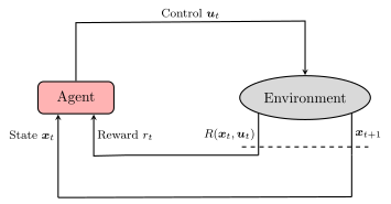
At a high level, most reinforcement learning algorithms follow the same basic learning cycle. First, the agent interacts with the environment by observing the state , applying an action from a chosen behavior policy††margin: The behavior policy does not necessarily have to match the learned policy . , and then observing the next state and scalar reward . This procedure, as illustrated in Figure 18.1, may repeat for multiple steps, during which the agent uses the observed transitions to update its policy.
18.1.2 Problem Formulation
Let us briefly revisit the MDP framework, which provides a standard mathematical formalization of the reinforcement learning problem. Formally, an MDP is defined as a tuple:
where denotes the state space, which is the set of all possible environment states and can be either discrete or continuous, denotes the action space, which is the set of admissible actions and can also be discrete or continuous, characterizes the system dynamics through the transition probability distribution , specifies the reward function, and is a discount factor that determines the relative importance of future rewards. From a reinforcement learning perspective, the goal is to learn a policy defined as a probability distribution over actions given states, . We will use the term trajectory to refer to a sequence of states and actions of length , given by:
where may be infinite. Given a policy , the induced trajectory distribution is:
| (18.1) |
where is the initial-state distribution. The reinforcement learning objective is to maximize the expected discounted cumulative reward under this trajectory distribution, namely:
| (18.2) |
An additional concept required to fully characterize is that of discounting. In particular, the discount factor is a scalar value in the range that determines the relative importance of future rewards, whereby a smaller will make the agent focus more on immediate rewards, while a larger will make the agent give more importance to future rewards. For example, in the limit case with , the agent will only consider immediate rewards, while in the case with , the agent will consider all future rewards equally. Mathematically, discounting is also crucial in ensuring that the sum of rewards in is finite even in the infinite horizon case with , such that if and the rewards are bounded, the sum of the rewards will be finite. In practice, the choice of is often problem-dependent, and it is common to use a value close to to ensure that the agent considers future rewards.
18.1.3 Value Functions and Bellman Equations
Almost all reinforcement learning algorithms involve estimating value functions. At its core, a value function is a function of state or state-action pairs that defines how good††margin: As defined in the previous section, value functions quantify quality in terms of expected cumulative future rewards. it is for the agent to be in a given state or to take a given action in a given state. Since the reward an agent expects to receive in the future depends on the actions it will take, the value function is inherently defined with respect to a particular policy .
We define the state-value function, , as the expected sum of future rewards when starting in state and following policy thereafter††margin: Throughout this chapter, we primarily consider the infinite-horizon case when referring to , although the same concepts extend to the finite-horizon case. :
| (18.3) |
Similarly, the action-value function, , is the expected return when starting in state , taking action , and then following policy thereafter:
| (18.4) |
A key property of value functions used in the context of reinforcement learning and dynamic programming is that they satisfy the Bellman equations. The Bellman equations describe a recursive relationship that decomposes the value of a state or state-action pair into the immediate reward and the value of the next state or state-action pair. Formally, for any policy and any state , the Bellman equation defines the following self-consistency condition:
| (18.5) |
where, to simplify notation, we have omitted the time index and used to denote the next state.
Similarly, the Bellman equation for the action-value function is:
| (18.6) |
Crucially, the value functions and are unique solutions to the Bellman equations.
In the remainder of this chapter, we show how we can use the Bellman equations to derive algorithms for estimating and approximating value functions, and how we can use these value functions to derive optimal policies.
Central to the solution of reinforcement learning problems are the notions of optimal policies and optimal value functions. The term optimal derives from the fact that value functions induce a partial ordering over policies, where a policy is said to be better than or equal to another policy if its value is no worse in every state. Formally, we write if and only if:
An optimal policy is a policy that is better than or equal to all other policies, such that for all policies . While the optimal policy does not need to be unique, all optimal policies share the same optimal value function , defined as:
Similarly, optimal policies also share the same optimal action-value function , defined as:
As discussed above, and are value functions for the optimal policy, thus, they must satisfy the Bellman equations with respect to the optimal policy. However, because and are the optimal value functions, the Bellman equations can be written in a policy-independent form. This is achieved by exploiting the fact that, under an optimal policy, the value of a state is equal to the expected return obtained by selecting the best available action in that state.
Formally, the Bellman equations for the optimal state-value function and action-value function—referred to as the Bellman optimality equations—can be derived by substituting the expectation over the policy from Equation 18.5 and Equation 18.6 with a maximization over actions, and are given by:
| (18.7) | ||||
| (18.8) |
Why are and so central to reinforcement learning? The key reason is that, once either of these functions is known, deriving an optimal policy is substantially simpler. In particular, an optimal policy can be derived by acting greedily with respect to the optimal value functions. For example, given the optimal state-value function , the optimal policy can be computed as:
| (18.9) |
That is, once is known, determining the optimal policy reduces to a one-step lookahead where, at each state, the agent selects the action that leads to successor states with the highest expected value.
Access to the optimal action-value function, , simplifies the process even further. For any state , we can obtain the optimal policy by selecting the action that maximizes :
| (18.10) |
Thus, by representing a function over states (or state-action pairs), the optimal value functions allow for the direct computation of the optimal policy.
18.2 Dynamic Programming Methods
As we introduced in the referenced item, the key idea of dynamic programming is to decompose a complex problem into simpler subproblems. This is achieved by using value functions to systematically organize and structure the search for optimal policies. In this section, we show how we can leverage dynamic programming algorithms in the context of reinforcement learning by turning the Bellman equations into iterative update rules for the estimation of value functions. In particular, we explore how to use dynamic programming ideas to derive algorithms for two distinct but interconnected tasks: prediction and control.
Definition 18.1 (Prediction).
In the context of reinforcement learning, we often refer to the task of estimating the value function for a given policy as prediction.
Definition 18.2 (Control).
In the context of reinforcement learning, we often refer to the task of finding the optimal policy as control.
18.2.1 Prediction: Policy Evaluation
We first consider the prediction problem of estimating the value function, , under a given policy . According to the Bellman equation in Equation 18.5, the value of a state under policy is defined as an expectation with respect to the policy and state transition model. For simplicity, we assume that the state transition model and policy describe probability distributions over discrete states and actions, respectively, which allows us to express the expectations in the Bellman equation as sums rather than integrals††margin: The extension to continuous states and actions is fundamentally equivalent and requires the replacement of summations with integrals. :
| (18.11) |
Policy evaluation is an iterative algorithm to solve the prediction problem. Consider a sequence of approximations to the value function, denoted as , where is an arbitrarily chosen initial guess††margin: Under the condition that any terminal state, occurring when in the finite-horizon setting or when the episode terminates in the infinite-horizon setting, must be assigned a value of zero. . Policy evaluation uses the Bellman equation in Equation 18.11 as an update rule, such that at iteration , the value function for all states is updated according to:
| (18.12) |
It is important to note that is a fixed point of the update rule in Equation 18.12 since the Bellman equation for ensures equality in this case. Moreover, under mild regularity conditions, it can be shown that the sequence of value functions converges to as . As we will see in the remainder of this chapter, the ideas described above are at the core of many reinforcement learning algorithms, including both model-based and model-free methods.
18.2.2 Policy Improvement
Having introduced an approach for solving the prediction problem, namely, estimating the value function under a fixed policy, we now turn to the problem of control, where the objective is to compute an optimal policy. To address the control problem, we rely on the policy improvement theorem, which provides a principled mechanism for transforming a given policy into a new policy that is guaranteed to be better than or equal to the original.
Consider two policies, and , such that for all states :
| (18.13) |
Then, the policy is guaranteed to be better than or equal to , such that:
Intuitively, if chooses actions that are at least as good—according to the action-value function of in Equation 18.13—as those prescribed by in every state (i.e., ), then following cannot result in worse long-term performance than continuing to follow .
Consider the greedy policy , which selects, in each state, the action that maximizes the action-value function associated with policy ††margin: In other words, the greedy policy performs a one-step lookahead using the current state-value function . :
| (18.14) |
By construction, this greedy policy satisfies the condition of the policy improvement theorem in Equation 18.13 and is therefore guaranteed to be better than or equal to the original policy. We refer to the process of constructing a new policy by greedily selecting actions with respect to the current value function as policy improvement.
Suppose now that the greedy policy is as good as the original policy , such that . From the definition of the greedy policy in Equation 18.14, we have:
Since , this expression is equivalent to the Bellman optimality equation in Equation 18.7. Therefore, the value function must equal the optimal value function, and the policy is therefore optimal.
In other words, policy improvement provides a systematic procedure for iteratively improving a policy using its value function, and it converges once the optimal policy is reached.
18.2.3 Control: Policy Iteration
The policy improvement theorem provides a concrete strategy to improve a policy by greedily selecting actions with respect to the current value function. In this section, we discuss how we use this strategy, in tandem with policy evaluation, to construct an algorithm for finding the optimal policy. We refer to this algorithm for finding the optimal policy as policy iteration. At a high level, the key idea of policy iteration is as follows: starting from a given policy , we first evaluate it to obtain its value function and then improve the policy using this value function to produce a new policy . The improved policy is subsequently evaluated to compute , which is in turn used to derive an improved policy . This alternating process of policy evaluation and policy improvement is repeated until the policy converges to the optimal policy.
More formally, policy iteration defines a sequence of monotonically improving policies by alternating between policy evaluation and policy improvement:
where PE denotes policy evaluation and PI denotes policy improvement. We outline the policy iteration algorithm in Algorithm 1.
Policy iteration is guaranteed to converge to the optimal policy and value function, given enough iterations. In practice, since the policy evaluation step is an iterative algorithm, we typically initialize the value function to the value function from the previous step of policy iteration. This can increase the speed of convergence since the value function does not typically change substantially between iterations.
Example 18.2.1 (Grid World Policy Iteration).
Explore an implementation of policy iteration for a simple grid-world environment in the repository
github.com/StanfordASL/pora-exercises in the notebook
ch18/policy_iteration.ipynb.
The grid-world environment is a simple grid with action space:
that has a set of absorbing states that get a reward of , and every other state gets a reward of . For this world, the state transitions are deterministic, so taking an action is guaranteed to result in moving in the desired direction (i.e. transition occurs with probability ), but we will consider a stochastic policy, . In the notebook for this example:
-
1.
Run the provided code to see how the policy evaluation algorithm updates for a simple random policy. Try playing around with the discount factor to see how it affects the value function.
-
2.
Take a look at the policy iteration algorithm code. Note that since we are considering a stochastic policy we use the softmax function:
to define the policy probability, where is the Boltzmann constant that when increased will decrease the entropy of the distribution for (i.e. as the policy will approach being deterministic). Play around with the value of to see how it affects the optimal value function.
18.2.4 Control: Value Iteration
One drawback of policy iteration is that it requires a full policy evaluation step at each iteration. As a result, the algorithm can be computationally expensive, since it must wait for the value function to converge before performing a policy improvement step, which only happens in the limit††margin: Several variants of policy iteration mitigate this cost by using truncated or approximate policy evaluation steps. . To address this limitation, value iteration provides an alternative approach that combines policy evaluation and policy improvement into a single step. Value iteration defines the following update rule:
| (18.15) |
Starting from an arbitrary initial value function , the sequence of value functions generated by value iteration is guaranteed to converge to the optimal value function .
Value iteration can be interpreted through the lens of the Bellman optimality equation, where the update in Equation 18.15 corresponds to applying the Bellman optimality operator from Equation 18.7 to the current value function . In contrast to policy iteration, which alternates between iteratively solving the Bellman equation for a fixed policy and performing a separate policy improvement step, value iteration directly applies the Bellman optimality equation at every iteration. We outline the complete value iteration algorithm in Algorithm 2.
Policy iteration and value iteration are two of the most foundational algorithms in reinforcement learning and are the basis for many modern reinforcement learning algorithms.
18.2.5 Inheriting the Limitations of Dynamic Programming
Dynamic programming methods, including policy iteration and value iteration, are powerful tools for solving MDPs. However, these methods also inherit the limitations of dynamic programming as they require a complete model of the environment, , to compute the expectations in the Bellman equations, and are computationally expensive for large state and action spaces. In the next sections, we discuss two key approaches to address these limitations. We first introduce sampling methods, which relax the requirement of having a complete model of the environment, and then we introduce the concept of function approximation, which helps address the computational complexity of dynamic programming methods.
18.3 Learning Paradigms for Model-free Control
In this section, we introduce two classes of learning methods that estimate value functions and compute optimal policies without requiring a complete model of the environment: Monte Carlo (MC) methods and temporal-difference (TD) learning. These methods are particularly effective in practice since they are applicable to a wide range of problems where modeling the environment dynamics is either impractical or infeasible. Similar to our discussion of dynamic programming methods, we first address the prediction problem for both Monte Carlo and temporal-difference methods before extending the analysis to the control problem.
18.3.1 Monte Carlo Methods
The term Monte Carlo broadly refers to a class of algorithms that rely on random sampling to estimate quantities of interest. In the context of reinforcement learning, Monte Carlo methods represent a class of approaches for solving the reinforcement learning problem based on averaging observed cumulative rewards from experience††margin: We often use the terms samples or experience to refer to sequences of states, actions, and rewards collected by interacting with the environment. . We assume that the agent interacts with the environment for a fixed number of time steps , referred to as an episode, during which it collects a trajectory consisting of states, actions, and rewards. Episodic MDPs naturally describe tasks with well-defined beginnings and endings, such as navigating a maze, playing a game, or completing a robotic assembly. At the end of each episode, the agent uses these observed trajectories to estimate quantities of interest, such as value functions or policy updates.
Monte Carlo methods for solving the prediction problem aim to learn the value function (or equivalently, ) given a policy . In this section, we first address the problem of using Monte Carlo methods for learning the state-value function , and then extend the discussion to learning the action-value function . Since the value of a state is defined as the expected cumulative reward obtained when starting from that state, it can be estimated by averaging the cumulative rewards observed across episodes that visit the state. As the agent visits a state more frequently, the estimate of its value becomes increasingly accurate.
Formally, suppose we wish to learn the value of the state under the policy , using a set of episodes passing through . The state-value function can be estimated using the Monte Carlo prediction procedure outlined in Algorithm 3.
In particular, Monte Carlo prediction updates the value estimate using the incremental update rule:
which moves the current estimate toward the observed return , where denotes the number of times state has been visited. This incremental form provides an efficient way to compute sample averages and is equivalent to the empirical mean:
where is the cumulative future reward observed in the -th visit to state .
We can also use Monte Carlo methods for learning action values††margin: Learning action values is useful in practice because we can use them to directly derive an optimal policy using Equation 18.10. . At a high level, Monte Carlo methods for estimating action value functions are essentially equivalent to the method presented above for estimating state values, with the only difference being that we now consider visits to state-action pairs instead of states. We consider a state-action pair to have been visited in an episode if the agent is in state and takes action at some point during the episode. As with state-value estimation, Monte Carlo methods estimate the action-value function by averaging the cumulative rewards observed from visits to the state–action pair . However, estimating action values introduces an additional challenge.
Suppose that experience is generated using a deterministic policy . Under such a policy, the agent selects the same action whenever it encounters a given state and therefore observes rewards for only one action per state. As a result, the agent receives no information about the values of alternative actions in that state, making it impossible to compare actions and improve the policy. This challenge is known as the problem of maintaining exploration and is central to reinforcement learning. As we will see throughout the remainder of this chapter, a common strategy for addressing this issue is to employ policies that ensure every state–action pair is visited with nonzero probability. One way to achieve this is by using stochastic policies that assign positive probability to all actions in each state, thereby guaranteeing sufficient exploration of the environment.
18.3.2 Temporal-Difference Learning
Temporal-difference (TD) learning is widely considered one of the most influential concepts in reinforcement learning. At a high level, temporal-difference learning combines elements of both Monte Carlo methods and dynamic programming. Like dynamic programming methods, temporal-difference learning updates value estimates using other learned estimates rather than waiting for complete returns. This mechanism is known as bootstrapping and allows learning from incomplete sequences of experience††margin: In other words, without waiting for the end of an episode. At the same time, like Monte Carlo methods, temporal-difference learning learns directly from sampled experience and does not require an explicit model of the environment: a property referred to as sampling. By combining bootstrapping with sampling, temporal-difference learning effectively bridges the gap between Monte Carlo and dynamic programming methods, inheriting many of the advantages of both approaches.
Similar to Monte Carlo methods, temporal-difference methods address the prediction problem by collecting samples from the environment and using them to update value estimates. Recall that in Monte Carlo methods, we must wait until the end of the episode to compute the cumulative reward following time , which we denote as , and then use to define the target for the value function update:
| (18.16) |
where denotes the assignment operator and is an externally-specified step-size parameter††margin: In Algorithm 3, we used . In contrast, temporal-difference methods update the value function estimate at each time step based on the observed reward and the estimate of the value function at the next state by the update:
| (18.17) |
This update rule is known as the TD() update, where the subscript indicates that the update relies on a single step of experience††margin: TD() is a special case of the more general TD() family of methods. . By comparing the Monte Carlo and temporal-difference update rules, we observe that computing the Monte Carlo target requires access to an entire episode, whereas the temporal-difference target can be computed immediately at each time step . We provide a complete algorithm for TD() in Algorithm 4.
It is worth noting that the quantity can be interpreted as an error that measures the discrepancy between the current estimate of the value function, , and an improved target estimate, ††margin: This target is more informative because it incorporates the realized reward from the transition , together with the current estimate of the value of the successor state. . This quantity, known as the TD error, plays a crucial role in the development of many reinforcement learning algorithms.
18.3.3 Example: Monte Carlo Control
We have already discussed how we can use the Monte Carlo and temporal-difference learning paradigms to address the problem of learning without a model of the environment. However, we solely discussed these methods in the context of the prediction problem, where we are trying to estimate the value function of a given policy. In this section, we introduce our first complete example of a reinforcement learning algorithm for learning optimal policies through Monte Carlo methods. Later in this chapter, we introduce various reinforcement learning algorithms that, in one way or another, build upon the principles of model-free control that we discuss here.
The central idea behind using Monte Carlo methods for control mirrors the principles underlying policy iteration, as introduced in Section 18.2. We use the term Generalized Policy Iteration (GPI) to refer to the broad framework encompassing all methods that alternate between policy evaluation and policy improvement. To illustrate this idea, consider a straightforward Monte Carlo extension of the classical policy iteration algorithm. Starting from an arbitrary initial policy , the algorithm alternates between two phases: policy evaluation, in which the value function of the current policy is estimated from sampled experience, and policy improvement, in which the policy is updated based on these value estimates. This process is repeated until convergence.
As discussed in Section 18.3.1, learning action-value functions is often more convenient than learning state-value functions, since action values can be used directly to derive policies. Accordingly, in this example we focus on learning the action-value function. At a high level, the algorithm proceeds by repeatedly alternating between the following steps:
where denotes policy evaluation, and denotes policy improvement. In contrast to the Policy Iteration algorithm, we use the Monte Carlo prediction approach from Section 18.3.1 in the policy evaluation step rather than using the exact Bellman equation to update the value function, which would require a model of the environment. The policy improvement step remains the same, where we define the new policy by acting greedily with respect to the current action-value function by choosing .
While this algorithm captures several core principles underlying many reinforcement learning algorithms, it remains relatively simplistic. As discussed in earlier sections, learning accurate action-value estimates from experience requires the agent to maintain sufficient exploration. More formally, the behavior policy must ensure that every state–action pair is visited with nonzero probability. In the formulation presented above, however, no explicit exploration mechanism is incorporated to guarantee this condition. As a result, the algorithm is only valid under the exploring starts assumption, which posits that each episode begins in every possible state–action pair with nonzero probability. Although useful for theoretical analysis, this assumption is generally unrealistic in practical applications. To obtain a practical and broadly applicable algorithm, this assumption must be relaxed. In the following sections, we introduce several strategies for ensuring adequate exploration, enabling effective learning from experience in realistic settings.
18.3.4 A Unifying View of Reinforcement Learning
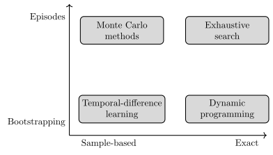
Monte Carlo, temporal-difference, and dynamic programming methods are often presented as distinct approaches to reinforcement learning. However, it is worth noting that these methods are extremes of a spectrum. To appreciate this, we can consider the advantages, disadvantages, and commonalities of each of these paradigms.
Monte Carlo and temporal-difference methods have an advantage over dynamic programming methods in that they do not require an explicit model of the environment and can learn directly from interaction with it—that is, they rely on sampling. This property greatly extends the applicability of these methods to real-world problems, where the environment could be unknown or too complex to model.
Temporal-difference and dynamic programming methods, in turn, offer a key advantage over Monte Carlo methods in that they update value estimates without waiting for an episode to terminate and can therefore learn from incomplete sequences of experience through bootstrapping. This capability is particularly important in practice, as many real-world tasks involve very long or even non-terminating episodes.
On the other hand, Monte Carlo methods also possess an advantage over temporal-difference methods in that they provide unbiased estimates of the true value function. This is because Monte Carlo updates rely on the actual return , whereas temporal-difference methods update toward an estimated target, . By doing so, temporal-difference methods deliberately trade some bias—arising from bootstrapped targets—for a reduction in variance, since these targets depend on fewer sources of stochasticity.
These relationships are summarized in Figure 18.2, which organizes reinforcement learning methods along two dimensions: the use of samples and the degree of bootstrapping. At the top right lies exhaustive search, where quantities of interest—such as value functions—are computed exactly through model-based simulation of all possible system evolutions. At the bottom right are dynamic programming methods, which leverage the principle of optimality and a known model to perform one-step lookahead updates via bootstrapping. Moving leftward relaxes the requirement of a model or exhaustive computation, replacing it with learning from sampled experience. At the top left are Monte Carlo methods, which avoid exhaustive search by learning from complete episodes. Finally, at the bottom left are temporal-difference methods, which combine the sampling of Monte Carlo methods with the bootstrapping of dynamic programming, enabling efficient learning from incomplete sequences of experience.
18.4 A Taxonomy of Reinforcement Learning
Over the last years, the field of reinforcement learning has seen a rapid growth in the number of algorithms and methods, each with its own strengths and weaknesses. While an exhaustive treatment of all these methods is beyond the scope of this chapter, we aim to provide an overall picture of the different types of algorithms that exist, a deeper understanding of the core principles that underlie these algorithms, and a number of representative examples from each category. In this section, we provide a bird’s-eye view of the field of reinforcement learning and classify the different algorithms into a taxonomy, shown graphically in Figure 18.3, that can serve as reference through the rest of the chapter.
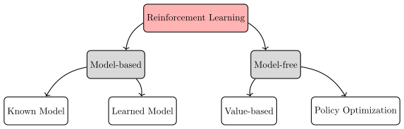
The first fundamental distinction among reinforcement learning algorithms is between model-free and model-based methods. Model-free methods, which are the focus of Section 18.5, attempt to learn the optimal policy directly from experience, without explicitly modeling the environment. Model-based methods, on the other hand, aim to learn a model of the environment and then use this model to derive optimal policies. We cover model-based methods in Section 18.6.
Looking at model-free methods, we can further distinguish between value-based and policy optimization methods. Value-based methods, similar to the ones described in previous sections, define the policy implicitly through a value function. By doing so, the main focus of value-based methods lies in accurately estimating the optimal value function, which we can then use to derive the optimal policy. Policy optimization methods, on the other hand, represent the policy explicitly via a parametric function and optimize the parameters of this function to maximize the reinforcement learning objective.
On the other side of the graph in Figure 18.3, we can see how model-based methods can be further divided into algorithms that either focus on learning a model of the environment from data, or algorithms that use a known model††margin: For example, the model could be known from physics or other domain knowledge. to derive optimal policies. In this chapter, we focus on methods that learn a model of the environment from data. As we will see in Section 18.6, learned models can be used in various ways, such as within planning routines or for accelerating model-free algorithms.
18.4.1 On-policy vs Off-policy Learning
Another crucial distinction among reinforcement learning algorithms is between on-policy and off-policy learning. On-policy methods aim to evaluate or improve the policy that is used to interact with the environment. Off-policy methods, on the other hand, evaluate or improve a policy that is different from the one used to interact with the environment. For example, the Monte Carlo control algorithm we presented in Section 18.3.3 is an on-policy method, as it attempts to improve the same policy used to make decisions in the environment. Off-policy methods define two distinct policies: one that must be updated and ideally becomes the optimal policy and one used to interact with the environment. We refer to the policy being learned as the target policy, while we refer to the policy used to generate samples from the environment as the behavior policy.
In general, on-policy methods are simpler to implement and tend to be more reliable than off-policy methods. Off-policy approaches, on the other hand, are typically more complex and require additional algorithmic considerations, which can make the learning phase less stable and lead to slower convergence in practice. Off-policy learning enables agents to learn from data generated by arbitrary behavior policies, including data collected by human demonstrators or by conventional, non-learning-based controllers. Moreover, off-policy methods make it possible to learn about multiple policies simultaneously, or to learn an optimal policy while continuing to explore the environment.
Throughout the next sections, we introduce various on-policy and off-policy methods for learning and discuss the advantages and disadvantages of each approach.
18.5 Model-free Reinforcement Learning
Model-free reinforcement learning methods are commonly considered to be the most popular and widely used class of algorithms in the field. This popularity is largely due to their recent successes in a wide range of applications, including playing games66. Silver, D., Huang, A., Maddison, C. J., Guez, A., Sifre, L., van den Driessche, G., Schrittwieser, J., Antonoglou, I., Panneershelvam, V., Lanctot, M., Dieleman, S., Grewe, D., Nham, J., Kalchbrenner, N., Sutskever, I., Lillicrap, T., Leach, M., Kavukcuoglu, K., Graepel, T., Hassabis, D. “Mastering the game of Go with deep neural networks and tree search.” Nature 529(7587), 484–489, 2016., robot control77. Levine, S., Finn, C., Darrell, T., Abbeel, P. “End-to-End Training of Deep Visuomotor Policies.” Journal of Machine Learning Research 17(39), 1–40, 2016., and the fine-tuning of large-scale AI chatbots88. Bai, Y., Jones, A., Ndousse, K., Askell, A., Chen, A., DasSarma, N., Drain, D., Fort, S., Ganguli, D., Henighan, T., Joseph, N., Kadavath, S., Kernion, J., Conerly, T., El-Showk, S., Elhage, N., Hatfield-Dodds, Z., Hernandez, D., Hume, T., Johnston, S., Kravec, S., Lovitt, L., Nanda, N., Olsson, C., Amodei, D., Brown, T., Clark, J., McCandlish, S., Olah, C., Mann, B., Kaplan, J. “Training a Helpful and Harmless Assistant with Reinforcement Learning from Human Feedback.” 2022.. In this section, we discuss representative reinforcement learning algorithms while maintaining our focus on key principles important for understanding and implementing new algorithms.
18.5.1 Value-based Methods
We begin our discussion on model-free reinforcement learning with value-based methods, which, similarly to the Monte Carlo control algorithm presented in Section 18.3.3, estimate the value function of a policy and use this estimate to derive the optimal policy.
Q-learning.
One of the first breakthroughs in reinforcement learning was the introduction of the Q-learning algorithm99. Watkins, C. J. C. H., Dayan, P. “Q-learning.” Machine Learning 8(3), 279–292, 1992.. Q-learning is an off-policy algorithm that learns the optimal action-value function via TD learning. Because Q-learning is off-policy, it estimates the optimal action value function independently of the behavior policy used to interact with the environment. The behavior policy therefore does not determine the objective of learning, but instead governs which state–action pairs are explored and, consequently, which action-value estimates are updated. Provided that the behavior policy is sufficiently exploratory††margin: That is, all state–action pairs are visited infinitely often in the limit. , Q-learning is guaranteed to converge to the optimal action-value function .
Given a transition sampled from the environment, , Q-learning updates the action-value estimate according to:
| (18.18) |
where is a tunable learning rate parameter. Importantly, regardless of the behavior policy used to generate the transition , the update in Equation 18.18 adjusts the current estimate toward the action value induced by the greedy policy with respect to the current Q-function, namely . In this sense, Q-learning repeatedly enforces the Bellman optimality equation for the action-value function until convergence††margin: As discussed in Section 18.2.4, the Bellman optimality operator has a unique fixed point, which corresponds to the optimal action-value function . . From this perspective, Q-learning can be viewed as a sample-based approximation of Q-value iteration††margin: That is, value iteration applied to action-value functions rather than state-value functions. , in which the Bellman optimality update is performed using a single transition sample.
To ensure that the behavior policy is sufficiently exploratory, Q-learning typically employs an -greedy action-selection strategy. Despite its simplicity, the -greedy policy approach is an effective and widely used exploration mechanism where, with probability , the agent selects the action that is greedy with respect to the current Q-function, while with probability it selects an action uniformly at random. This strategy ensures that for all states and actions , which is a key requirement for the convergence of Q-learning. We present the complete Q-learning algorithm in Algorithm 5.
Value Function Approximation.
So far, we have assumed that the state and action spaces, and , are finite and small enough to be easily stored in a look-up table and to allow for meaningful state-action space exploration within a reasonable computation budget. However, in robotics applications, the state and action spaces are often continuous or extremely high-dimensional, making it impractical to compactly store and efficiently update value functions. This challenge motivates us to consider methods that rely on parametrized function approximation. Within this class of methods, we represent value functions by a parametric function, , or alternatively , with parameters . The goal of learning is then to find the optimal parameters , such that the value function estimator is close to the optimal value function.
Function approximation has two key advantages. First, it allows us to represent value functions compactly, as the number of parameters is typically much smaller than the number of states and actions. Second, it enables the value function estimator to generalize to unseen states and actions, potentially reducing the amount of exploration required to learn a good policy††margin: In other words, if the function approximator is able to generalize successfully, the agent does not need to visit every state-action pair. . While there are many choices for the function approximator, including linear functions, neural networks, and decision trees, we focus our discussion on differentiable functions.
Given a dataset, , of transitions , policy evaluation via function approximation entails learning the parameters that minimize the loss function :
| (18.19) |
Intuitively, measures the discrepancy between the estimated value function, , and the target value function, , where is the value function under the policy that generated the transitions in . This optimization problem can be solved via stochastic gradient descent, which defines the following update rule:
| (18.20) |
where:
Here, denotes the gradient of the value function estimator with respect to its parameters , and is the learning rate.
In practice, however, the update rule in Equation 18.20 is not directly applicable since the true target value function is unknown. Leveraging ideas from model-free control, the unknown target can be replaced by an estimate derived from Monte Carlo, temporal-difference, or dynamic programming methods. For example, using a Monte Carlo estimate, the parameter update can be written as:
| (18.21) |
where denotes the return observed from time step . Alternatively, a temporal-difference approach replaces the Monte Carlo return with a one-step bootstrap estimate, yielding the update:
| (18.22) |
In both cases, the Monte Carlo and temporal-difference targets are computed from trajectories generated by applying the behavior policy in the environment.
Fitted Q-learning.
A particularly popular algorithm that combines function approximation with temporal-difference learning is the Fitted Q-Learning algorithm. Fitted Q-Learning updates the parameters of a Q-function estimator by applying the update rule in Equation 18.20 with:
| (18.23) |
It is important to note that the target is equivalent to the temporal-difference target used in Q-learning. Essentially, Fitted Q-Learning mimics the update rule of Q-learning, but rather than directly updating the action values to explicitly enforce the Bellman optimality equation it updates the parameters of the Q-function estimator to approximately enforce it. In other words, rather than updating the entries of a look-up table representing the value function, Fitted Q-learning updates the parameters to minimize the error with respect to the fixed point of the Bellman optimality operator.
In this section, we discussed a few foundational examples of value-based reinforcement learning methods. While these are only a subset of the vast literature in value-based methods, they convey the key ideas and challenges of learning value functions for control. Specifically, these methods highlight the central idea of approximating value functions from experience and leveraging them to derive optimal policies. Key challenges include ensuring sufficient exploration, which we can address through strategies like -greedy policies, and addressing stability and convergence of the learning process when using value function approximators, particularly in high-dimensional or continuous spaces. Value-based methods in reinforcement learning are fundamentally built on a concise set of core principles, such as generalized policy iteration and (approximate) value iteration, and differ primarily in their usage of value update targets††margin: For instance, Monte Carlo, temporal-difference, or dynamic programming approaches. , function approximators, or behavior policies. Therefore, understanding these foundational concepts provides us a lens through which we can interpret the majority of value-based algorithms.
18.5.2 Policy Optimization Methods
We now continue our discussion of model-free reinforcement learning by turning to policy optimization (PO) methods. In contrast to value-based approaches, policy optimization methods adopt a fundamentally different strategy for solving the reinforcement learning problem by directly optimizing the policy itself. To better motivate policy optimization, let us recall the reinforcement learning objective from Section 18.1:
Rather than learning a value function and deriving a policy from it, as in value-based methods, policy optimization methods define a parametric policy, , and directly optimize the parameters to maximize the reinforcement learning objective . Formally, the goal of policy optimization is to find the optimal policy parameters:
| (18.24) |
where, for simplicity, we use to refer to the reinforcement learning objective, , under policy with parameters .
Policy optimization methods typically address this problem in two stages. First, they estimate the gradient of the objective with respect to the policy parameters, . Then, they update the parameters by performing (approximate) gradient ascent:
| (18.25) |
where is a user-defined learning rate.
The first challenge that all policy optimization methods face is estimating the gradient of the reinforcement learning objective. To simplify the notation, we define the cumulative reward as and assume ††margin: The extension to the discounted case is equivalent and relatively straightforward. . By definition of expectation, we have:
| (18.26) |
where denotes the trajectory distribution induced by the policy . Equation 18.26 allows us to write the gradient of the reinforcement learning objective as:
| (18.27) |
However, we cannot compute this gradient directly because it depends on unknown dynamics through the trajectory distribution, ††margin: Recall that we do not assume access to the system dynamics and thus cannot compute explicitly. .
To address this issue, we resort to the following useful identity:
| (18.28) |
and use it to rewrite the gradient of the reinforcement learning objective in Equation 18.27 as:
We can then approximate the expectation using Monte Carlo methods by sampling from the trajectory distribution, , through interaction with the environment. However, the gradient of the log-probability, , remains intractable to compute directly. To address this, let us recall the definition of the trajectory distribution, :
| (18.29) |
where taking the logarithm yields:
| (18.30) |
By substituting Equation 18.30 into the gradient of the reinforcement learning objective, we obtain:
Notably, the terms and do not depend on , and thus can be ignored when computing the gradient of the reinforcement learning objective. Moreover, evaluating the gradient of the log-probability of the action, , is tractable and we can easily compute it, for example by using automatic differentiation tools.
This leads to the following expression for the gradient of the reinforcement learning objective:
| (18.31) |
which is tractable to compute and which we can estimate using samples from the environment. For example, given episodes of interaction with the environment, we can estimate the gradient of the reinforcement learning objective as:
| (18.32) |
This is a crucial result and lays the foundations for almost all policy optimization algorithms in reinforcement learning.
REINFORCE.
The derivations above directly lead to one of earliest examples of policy optimization methods††margin: In the reinforcement learning literature, these are often also referred to as policy gradient methods. known as the REINFORCE algorithm1010. Williams, R. J. “Simple statistical gradient-following algorithms for connectionist reinforcement learning.” Machine Learning 8(3), 229–256, 1992.. At a high level, the REINFORCE algorithm estimates the gradient of the reinforcement learning objective in Equation 18.32 using samples from the environment, and after each episode updates the policy parameters in the direction of the gradient. We outline the REINFORCE algorithm in Algorithm 6.
From Equation 18.31, we can see that the gradient is computed as the sum of the gradients of the log-probabilities of the actions, weighted by the return of the trajectory. Although this result follows from a mathematical derivation, it also admits a clear and intuitive interpretation. By updating the policy parameters in the direction of the policy gradient, the algorithm increases the log-probability of actions that lead to high returns while decreasing the log-probability of actions that lead to low returns. In this way, the policy gradient formalizes the notion of trial-and-error learning, where behaviors that prove effective are reinforced, whereas ineffective behaviors are gradually suppressed.
Policy optimization methods represent a popular and intuitive approach to reinforcement learning and have several advantages and disadvantages compared to value-based methods. A first key advantage of policy optimization methods is that they can naturally handle both discrete and continuous action spaces because we can compute the gradient of the policy using automatic differentiation tools††margin: Assuming the policy is parameterized by a differentiable function. . For example, in the case of continuous action spaces, we can parameterize the policy as a Gaussian distribution, and all of the derivations developed in this section would still hold. Additionally, policy optimization methods have the notable advantage of directly optimizing the reinforcement learning objective. This ensures that improvements to the policy are measured against a well-defined metric, since better values of the reinforcement learning objective imply a better policy. In contrast, value-based methods rely on fixed-point iterations of value functions to satisfy the Bellman equation with the goal to eventually converging to the optimal value function. While this approach is theoretically sound, it is unclear how suboptimal the policy is during intermediate iterations.
Policy gradient methods also have some disadvantages. First, the policy optimization methods presented so far are inherently on-policy methods, which can result in high sample inefficiency††margin: A number of off-policy policy optimization algorithms have been introduced to allow the policy to be updated using experiences collected from different policies. These methods aim to approximate the behavior of classical on-policy algorithms while improving sample efficiency. Despite this advantage, they often introduce additional complexities, such as the need for more sophisticated exploration strategies and managing the stability of the off-policy updates. . A second disadvantage is that the gradient defined in Equation 18.32 is a high-variance estimator of the true gradient from Equation 18.31. In practice, this can lead to extremely noisy updates and therefore slow convergence.
As we will see in the remainder of this section, a lot of research in the domain of policy optimization has focused on addressing these limitations to develop sample-efficient and lower-variance policy gradient estimates.
Actor-Critic Methods.
Actor-critic methods represent an important extension of policy optimization that reduces the high variance associated with policy gradient estimates. Let us recall the definition of the policy gradient and slightly rearrange the summation terms to highlight the sum over future rewards111Where again, for simplicity, we assume .:
We refer to the term as the reward-to-go. The reward-to-go is a one-sample estimate of the true return, which is defined as the expected cumulative reward under the trajectory distribution, . While conceptually straightforward, this reward-to-go estimate introduces significant variance, leading to noisy policy gradient updates.
Actor-critic methods address this challenge by introducing a critic, which is a parametric approximation of the value function. Since the value function estimates the expected reward-to-go, the critic enables us to replace the high-variance sample-based estimate with a lower-variance, learned approximation. Concretely, the policy gradient becomes:
| (18.33) |
where is the critic’s estimate of the action-value function. We can update the critic using any value estimation method, such as the value-based methods with function approximation discussed in Section 18.5.1.
A particularly popular choice for the definition of the policy gradient in actor-critic methods is through the advantage function:
| (18.34) |
which quantifies the relative merit of taking action in state , compared to the average value of the state. Intuitively, if the policy gradient in the REINFORCE algorithm can be thought of as a way to increase the probability of good actions, the advantage function can be thought of as a way to increase the probability of actions that are better than the average. This normalization of the policy gradient through the advantage defines the so-called Advantage Actor Critic (A2C) 1111. Mnih, V., Badia, A. P., Mirza, M., Graves, A., Lillicrap, T., Harley, T., Silver, D., Kavukcuoglu, K. “Asynchronous Methods for Deep Reinforcement Learning.” In Proceedings of The 33rd International Conference on Machine Learning, 1928–1937, 2016. algorithm, which significantly reduces variance and improves learning stability. In practice, we often approximate the advantage function to avoid estimating both and , using:
| (18.35) |
Actor-critic methods typically involve iterative updates of both the policy parameters, , and the value function parameters, . At each step, we improve the policy based on the estimated advantage and we refine the value function to better approximate future rewards. The pseudocode for A2C is presented in Algorithm 7 and highlights these alternating updates.
Actor-critic methods blend the strengths of policy optimization and value-based approaches, achieving a balance between expressive policy representations and efficient variance reduction. However, the introduction of a critic also adds computational complexity and tuning challenges that we must consider in practical implementations.
18.5.3 Limitations of Model-free Reinforcement Learning
Despite their successes, model-free reinforcement learning methods face several important challenges. A primary limitation is sample efficiency. Model-free algorithms often require a large number of interactions with the environment to learn an effective policy, which can be prohibitively expensive or impractical in many real-world settings, particularly in robotics. A second limitation is that, in their standard formulation, model-free methods are inherently single-task learners. Given a fixed reward function defining a specific task, these methods learn a policy optimized exclusively for that task, making it difficult to reuse knowledge or transfer learned behaviors across tasks. Finally, many real-world applications provide reward signals that are sparse, delayed, or noisy. Such reward structures significantly represent a challenge to the learning process, as useful feedback may be infrequent or difficult to attribute to specific actions. As a result, model-free methods can struggle to discover effective policies in these environments.
18.6 Model-based Reinforcement Learning
Model-based reinforcement learning methods aim to address the limitations of model-free methods by learning a model of the environment. In this section, we introduce two broad classes of model-based reinforcement learning methods: model-based planning methods that learn a model and use it to plan and model-based policy optimization methods that learn a model and use it to accelerate model-free policy learning.
18.6.1 Model-based Planning
If we had access to a model of the dynamics, , we could directly leverage tools from model-based optimal control to compute an optimal action sequence or policy. Motivated by this observation, the central idea behind model-based planning methods is to learn an approximate model of the environment dynamics from data, and then use this learned model to plan.
A generic model-based planning procedure can be summarized as follows:
-
1.
Run a base policy, , in the environment and collect a dataset of transitions, .
-
2.
Fit a dynamics model, , to the observed data to minimize the prediction error, for example by minimizing the mean squared error between the predicted and true next state:
-
3.
Use the learned dynamics model to plan a sequence of actions for the agent to execute.
Despite its simplicity, this scheme works for relatively well-behaved systems, where the dataset guarantees sufficient coverage of the state-action space, and where the learned model is accurate enough to enable effective planning††margin: This scheme is essentially equivalent to a task known as system identification. . However, in practice, learning an accurate model of the dynamics is often challenging, especially when dealing with high-dimensional, non-linear, and stochastic systems. Most importantly, inaccuracies in the learned model are particularly problematic when used within an optimization process. Optimization algorithms will naturally exploit inaccuracies in the model that have high predicted performance, but may not correspond to high realized performance.
A popular approach to address this issue is to consider a measure of uncertainty in the model’s predictions, and to use this uncertainty to inform the planning process. While there are many ways to quantify uncertainty, we consider methods that aim to learn a posterior distribution over the model parameters. In these methods, rather than learning a single estimate of the model parameters through standard maximum likelihood estimation:
| (18.36) |
where is the likelihood of the data given the model parameters, we instead aim to learn a posterior distribution, , over the model parameters. In other words, we aim to learn a full distribution over the model parameters that is consistent with the observed data, potentially capturing multiple plausible models that explain the data, and ultimately enabling us to reason about the uncertainty in the model’s predictions. We can achieve this by applying Bayes’ rule to compute the posterior distribution:
| (18.37) |
where is the likelihood of the data given the model parameters, is the prior distribution over the model parameters, and is the marginal likelihood of the data. While a complete treatment of Bayesian inference is beyond the scope of this book, we refer the interested reader to standard textbooks on the subject, such as by Murphy (2022)11. Murphy, K. P. Probabilistic Machine Learning: An introduction. MIT Press, 2022.. For the purpose of this chapter, it will be sufficient to assume that Bayesian inference provides us with computational methods to derive an estimate of the posterior distribution, which we can then use to inform the planning process.
Once we have an estimate of the posterior distribution over the model parameters, we can apply it in the following model-based planning scheme:
-
1.
Run a base policy, , in the environment and collect a dataset of transitions, .
-
2.
Use to estimate a posterior distribution, , over the model parameters.
-
3.
Sample a set of plausible models, .
-
4.
For each sampled model, , and given a candidate action plan, , use the model to compute the expected return:
where .
-
5.
Execute the first action from the best plan according to the expected return.
This scheme allows us to leverage the uncertainty in the model’s predictions by considering multiple plausible models and to reason about the expected return under each model rather than optimizing under a single model.
Despite its effectiveness, it is important to note that this scheme is just a high-level description of the model-based planning process, and there are many practical considerations that we would need to address to make this approach work in practice.
18.6.2 Model-based Policy Optimization
The second class of model-based reinforcement learning methods we consider is model-based policy optimization. In contrast to model-based planning, which uses the learned model to plan a sequence of actions, model-based policy optimization uses the learned model to improve model-free policy learning.
Specifically, having a learned model allows us to consider two sources of experience: real-world data collected by executing the policy in the environment and synthetic data generated by the model. Given an MDP, , and a learned model, ††margin: Here we consider the general case where we learn both the next state and the reward, but we can extend the discussion to the case where we only have to learn one of the two. , we can consider two sources of experience:
The basic idea of model-based policy optimization is to use both sources of experience to improve model-free policy learning. One of the earliest and most popular methods in this category is the Dyna-Q algorithm1212. Sutton, R. S. “Dyna, an integrated architecture for learning, planning, and reacting.” SIGART Bull. 2(4), 160–163, 1991..
Dyna-Q.
The Dyna-Q algorithm is a model-based reinforcement learning algorithm that improves the learning efficiency of Q-learning by using the learned model to generate synthetic data††margin: The term Dyna-Q derives from the fact that the algorithm combines Q-learning with model-based acceleration. The term Dyna more generally refers to the idea of using a learned model to generate synthetic data for model-free learning. . The algorithm is based on the idea that in addition to updating the Q-function using real-world data, we can also update the Q-function using synthetic data generated by the learned model. At a high-level, the algorithm alternates between three main steps. First, it performs standard Q-learning updates, using real experience collected from interactions with the environment to update the Q-function. Second, it carries out a model learning step, in which the dynamics model is updated based on the same real-world data. Finally, the algorithm executes a model-based acceleration step, during which the learned model is used to generate synthetic experience that is then leveraged to perform additional Q-function updates. A detailed description of this algorithm is provided in Algorithm 8.
The Dyna-Q algorithm is a simple yet powerful method that demonstrates the potential of model-based reinforcement learning to improve the learning efficiency of model-free algorithms.
18.6.3 Limitations of Model-based Reinforcement Learning
Model-based methods are an extremely active and promising area of research in reinforcement learning, but they are also subject to several limitations. First, model learning entails optimizing the parameters of the model to minimize prediction error. However, this objective does not necessarily align with the objective of the agent, which is to maximize the expected cumulative reward, and this discrepancy can lead to suboptimal policies. Second, model-based methods are sensitive to model errors, which can cause the agent to learn suboptimal policies or exploit the model errors to achieve high rewards, potentially leading to catastrophic failures. Finally, learning an accurate model of the environment is a challenging task, especially in complex environments with high-dimensional state and action spaces.
18.7 Summary
In this chapter, we provided a comprehensive overview of the field of reinforcement learning. Rather than presenting an exhaustive list of algorithms, we focused on a conceptual understanding of the key ideas and principles that underlie reinforcement learning. In particular, we discussed how Monte Carlo methods and temporal-difference learning represent two foundational paradigms in reinforcement learning, and how we can use these methods to estimate value functions and learn optimal policies. Most importantly, we highlighted how these methods, together with dynamic programming, define a full spectrum of possible approaches to the problem of learning from interaction. Finally, we also discussed concrete examples of the main algorithmic families in reinforcement learning, including model-free and model-based methods, and highlighted the key ideas behind some of the most popular algorithms within these categories.
To learn more.
For readers interested in a deeper exploration of the topics covered in this chapter, several authoritative resources are available. The definitive reference in the field is the textbook by Sutton and Barto (2018)22. Sutton, R., Barto, A. Reinforcement learning: An introduction. MIT Press, 2018., which provides a comprehensive and accessible introduction to the core principles of reinforcement learning, including Monte Carlo methods, temporal-difference learning, and function approximation. For a more rigorous treatment of the subject that emphasizes the connections between reinforcement learning, dynamic programming, and optimal control, we refer the reader to Bertsekas (2019)33. Bertsekas, D. Reinforcement learning and optimal control. Athena Scientific, 2019..
18.8 Exercises
The starter code for the exercises provided below is available online through GitHub. To get started, download the code by running in a terminal window:
We denote Problems requiring hand-written solutions and coding in Python with ![[Uncaptioned image]](/book-assets/reinforcement-learning/figs__write.png) and
and ![[Uncaptioned image]](/book-assets/reinforcement-learning/figs__code.png) , respectively.
, respectively.
Problem 1: Q-learning Widget Sales
You are the owner of Widget Co., a shop in the business of buying widgets wholesale and selling them to consumers at a markup. The shop is able to store between 0 and 5 widgets at a time, and we denote the number of widgets held in the shop on day as . Every day, you choose how many widgets to order from your supplier. You can order either zero widgets, a “half order” of widgets, or a “full order” of widgets. We write the number of widgets ordered to arrive on day as . A random number of customers (following an unknown distribution, though this distribution may be assumed to be consistent across all days) come to Widget Co. every day; each customer buys a widget if there are any available. We write the demand on day as , and assume . At the end of each day, you record a net profit for that day.
In this exercise, we will explore using Q-learning to help model returns and optimize the shop’s performance.
In the notebook for this exercise,
ch18/exercises/widget_sales.ipynb, complete the following:
-
1.
We have a dataset containing records for each day of the last three years of the shop’s operation. In the provided notebook, fill in the function q_learning to implement a -learning algorithm to learn tabulated -values from this dataset.
-
2.
Suppose you find that the dynamics of the number of widgets in the shop each day are described by:
and the daily net profit is:
where is the price you set for each widget, is the fixed rent on your shop, is the cost for storing each widget overnight, and is the cost of ordering widgets from your supplier. The quantity is the “satisfied demand” on day .
Let’s also suppose that after a few weeks of sales, you determine that the daily demand distribution for your widgets seems to be:
In the function action_value_iteration, implement value iteration to learn tabulated -values from the model described above. Specifically, use the following update equation:
which is a slight variation of Equation 18.15 for learning -values adapted for this problem’s model (see also Equation 18.8). Compare the -values from -learning compared to those from value iteration. What do you notice about the learned -values compared to those from value iteration? Why do you think this occurs?
-
3.
Finally, compute an optimal policy based on the -learning approach from the first part, and another optimal policy based on the value iteration part. Run the provided code to simulate each one over five years, and compute the cumulative profit for each day and for each optimal policy. Compare the cumulative profits over time. What do you notice about the difference between the two cumulative profit trends? Why do you think this occurs?
Problem 2: Cart-pole Balancing via Model-free Reinforcement Learning
In this problem, we will return to the classic “cart-pole” balancing control problem where our goal is to design a controller to balance an inverted pendulum upright on a cart. We have already explored this problem in the context of model-based optimal control (specifically LQR control) in a Chapter 3 exercise, but in this exercise we will approach the problem through model-free reinforcement learning.
To summarize the environment setup, the agent observes the state of the environment as , where denotes the horizontal position of the cart and denotes the angle of the pendulum from the upright position. At each instant, the agent chooses an action indicating whether to push the cart to the left or to the right ††margin: Note this is slightly different from the exercise in Chapter 3 where the control was the horizontal force on the cart. .
This exercise is split up into several parts, and the starter code can be found in the notebook ch18/exercises/cartpole_balance.ipynb.
-
1.
First, you will implement a deep Q-learning algorithm with experience replay, originally introduced in “Playing Atari with Deep Reinforcement Learning”1313. Mnih, V., Kavukcuoglu, K., Silver, D., Graves, A., Antonoglou, I., Wierstra, D., Riedmiller, M. A. “Playing Atari with Deep Reinforcement Learning.” ArXiv abs/1312.5602, 2013.. You can find the code for this part in q_learning.py:
-
(a)
Implement the function QLearning.build_network to create a model for the Q-function that takes as input a state vector and outputs a vector of Q-values for that state and each action.
-
(b)
Implement the function QLearning.policy_train that will be used to compute actions during the training process. Implement an -greedy approach that samples a random action with probability to ensure exploration.
-
(c)
Implement the functions QLearning.compute_target and QLearning.train to sample episodes and train the model using experience replay, see Algorithm 9 for the training algorithm.
-
(d)
Use the provided code to start training with your choice of hyperparameters.
Data: Initial action-value model, , parameterized by , number of episodesResult: Improved action-value model/* Initialize replay buffer */for to doInitialize .for each step of episode doif thenelseExecute , observe reward and next state .Sample random minibatch of transitions fromfor sample in minibatch doif is terminal thenelseUpdate model parameters, , using gradient descent on .returnAlgorithm 9 Deep Q-learning with Experience Replay -
(a)
-
2.
Next, you will implement the REINFORCE algorithm introduced in Section 18.5.2. Specifically, in this exercise you will implement three variations of the REINFORCE algorithm with slightly different definitions of the policy gradient, one of which is the standard version from Algorithm 6. You can find the code for this part in reinforce.py:
-
(a)
Implement the function Reinforce.build_network to create a model for the policy that takes as input a state vector and outputs a vector of action probabilities.
-
(b)
Implement the function Reinforce.policy_train that will be used to compute actions during the training process, as well as the value for the chosen action.
-
(c)
Implement the function Reinforce.train to sample episodes and train the model using the outline in Algorithm 6. Here, you will implement options for three different policy gradient definitions (i.e. ). First, implement the standard REINFORCE algorithm where the objective gradient is estimated using:
based on an episode sampled from the environment and is the total discounted reward of the episode.
Next, implement the policy gradient with a “causality trick”. This trick avoids reinforcing actions taken later in the episode based on rewards obtained early in the episode, since those later actions would have no causality in receiving earlier rewards. Specifically, with this trick you will compute the gradient estimate as:
where the term is the discounted reward-to-go from time .
Finally, you will implement a policy gradient that uses the “causality trick” with a “baseline”. The baseline helps to reduce the variance of the policy gradients by “centering” their returns. Specifically, compute the policy gradient as:
where the baseline is the average of the reward-to-go values over the episode. You can additionally scale the baseline by the inverse of the standard deviation of the reward-to-go values.
-
(d)
Use the provided code to start training with your choice of hyperparameters. What differences do you observe between the deep Q-learning algorithm and the REINFORCE algorithm in terms of performance during and after training? Which method is more sample efficient, and why? How do the different versions of the policy gradient compare within the REINFORCE method?
-
(a)
Problem 3: Advantage Actor Critic
As discussed in Section 18.5.2, actor-critic methods are a popular variance reduction technique for policy optimization. These methods use a value function as a baseline (the “critic”) and the learned policy is the “actor”. In this problem, you will implement key parts of the Advantage Actor-Critic (A2C) algorithm, which we described in Algorithm 7.
In the file ch18/exercises/advantage_actor_critic.ipynb, complete the following tasks:
-
1.
Using the model components already provided, write the code that implements the complete model, consisting of a couple linear layers to transform the input before being passed to heads for the policy and the value function (i.e. for the actor and critic). For the actor, the model outputs mean and standard deviation parameters for a multivariate normal distribution.
-
2.
For this implementation of A2C, we will use a Monte Carlo estimate to produce value targets for the critic, denoted by in Algorithm 7. To compute the Monte Carlo value target, implement the function to compute the discounted returns:
for an episode. What is the advantage of using Monte Carlo estimates over temporal-difference estimates in terms of the bias-variance tradeoff?
-
3.
Then, implement the function to compute the training loss for an episode:
where is the advantage and where the first term is the actor loss and the second (quadratic) term is the critic loss. Note that we are using JAX to compute gradients of the training loss with respect to the model parameters. When computing the training loss for the actor component, its important to use jax.lax.stop_gradient to stop JAX from backpropagating gradients in this term. Why is this important?
-
4.
Finally, run the provided code to train the model for a toy lunar lander environment.
Practice · 4 notebooks
- Advantage Actor Critic Open in Colab Source
- Cartpole Balance Open in Colab Source
- Widget Sales Open in Colab Source
- Policy Iteration Open in Colab Source