Modeling Robot Dynamics · Principles of Robot Autonomy

Robots can take on a wide variety of forms: they may have rigid or flexible structures, rely on different types of actuators for control, perceive their surroundings through diverse sensing modalities, or even exist as purely virtual agents. Despite this variety of embodiments, nearly all robotic systems share a fundamental characteristic—they are dynamic agents whose states evolve over time. The most immediate example of robot dynamics is physical motion, encompassing changes in position, velocity, joint configurations, and sensor orientations. A deep understanding of the dynamical properties of a robotic system is essential to its effective design and control. For instance, building a bipedal robot capable of walking or running requires detailed modeling of its motion to ensure that the mechanical structure and actuators can withstand the forces and torques involved. Accurate dynamic models are also critical for designing control strategies that achieve stable, efficient, and responsive locomotion.

This chapter introduces several foundational topics in modeling robotic systems. We will start with Section 1.1 by introducing the concept of a state space model, which provides a mathematical framework to describe the behavior of a robot’s state over time. Next, in Section 1.2, we will detail how a robot’s kinematics and dynamics are used to derive these state space models, focusing on the principles that govern physical motion and constraints. We will then explore specific motion models for wheeled robots in Section 1.3, including the unicycle and differential drive models, to illustrate practical applications of these concepts. Finally, in Section 1.4, we will discuss computational techniques for simulating robot dynamics, emphasizing numerical integration methods such as the Euler and Runge-Kutta methods to approximate and analyze the time evolution of robotic systems.

1.1 State Space Models

A state space model is a mathematical framework for describing the behavior of a dynamical system. Every state space model consists of two key components: a state and a model.

Definition 1.1 (State).

The state of a dynamical system at time $t_{0}$ is a minimal set of variables $\bm{x}(t_{0})$ such that, given the control input $\bm{u}(t)$ for all $t\geq t_{0}$ , the future evolution of the system’s state $\bm{x}(t)$ for all $t\geq t_{0}$ is uniquely determined, independently of the system’s behavior for $t<t_{0}$ .

Formally, the state is a sufficient statistic of the system’s history: given the current state and the external inputs to the system, the system’s future behavior is fully determined, independently of how that state was reached. The state of a robotic system can be finite or infinite-dimensional. For example, a simple mobile robot with a rigid body can be represented by a finite and low-dimensional state (e.g., the position and velocity of its center of mass), whereas a flexible robot might require an infinite-dimensional state to describe the continuous deformation of its body (e.g., a deflection function that describes the displacement at every point along the robot’s length).

When modeling the dynamics of a robot, it is important to define the state in a way that aligns with the specific goals and requirements of the application. In practice, the complexity of the state representation can often be reduced by omitting parts of the robot’s dynamics that are irrelevant to the problem at hand. For instance, in developing software to enable an autonomous car to navigate urban environments, it may be sufficient to model only its position, orientation, and velocity, while abstracting away the internal mechanics of the engine, tires, or suspension. Conversely, if the car is being designed for high-performance racing, these specifics become critical to accurately capture and optimize its behavior. Throughout this book, we focus on applications where the state is finite-dimensional and represent it as a vector $\bm{x}\in\mathbb{R}^{n}$ , referred to as the state vector.

The second key component of a state space model is the model itself, which defines the rules and equations governing the evolution of the state over time by relating it to a set of inputs and outputs.

The inputs to a model refer to external factors or control signals that influence the behavior of the system.^†^†margin: The term input is used interchangeably with control and action in different domains of robotics. These can include forces, torques, voltages, commands, or any other external stimuli that drive the system’s dynamics. As with the state, the dimensionality of the input may vary, but throughout this book we assume the input is represented by a finite-dimensional vector, $\bm{u}\in\mathbb{R}^{m}$ .

The outputs of a model are the observable variables or measurements derived from the system. These typically come from sensors or other measurement devices that capture data reflecting the system’s state and behavior. For example, a robot equipped with a global navigation satellite system (GNSS) sensor may directly measure its position but not its heading. In some cases, the relationship between the state and the output is complex—for example, the connection between a robot’s inertial pose and a red-green-blue-depth (RGB-D) camera image. The process of inferring the state from the outputs is referred to as state estimation, and it will be explored in detail in Chapters Chapter 11 - Chapter 15. We assume the output is finite-dimensional and denote it by the vector $\bm{y}\in\mathbb{R}^{q}$ .

Definition 1.2 (Model).

A model describes the evolution of a dynamical system through two types of equations: state equations and observation equations. The state equations specify how the state evolves as a function of the current state and inputs, while the observation equations define how the state influences the measurable outputs.

State equations are typically modeled as differential equations^†^†margin: Ordinary differential equations are most commonly used to model robotic systems. However, partial differential equations may be needed for more complex cases, such as systems with flexible or deformable structures, where dynamics vary over both space and time. describing the changes in the state with respect to an independent variable, usually time:

\dot{\bm{x}}=f(\bm{x}(t),\bm{u}(t)),

(1.1)

where $\dot{\bm{x}}=\frac{d\bm{x}(t)}{dt}$ is the time derivative of the state vector $\bm{x}(t)$ , and $f\colon\mathbb{R}^{n}\times\mathbb{R}^{m}\to\mathbb{R}^{n}$ is the dynamics function of the system.

Observation equations take the form:

\bm{y}(t)=h(\bm{x}(t),\bm{u}(t)),

(1.2)

where $\bm{y}(t)$ denotes the output at time $t$ , and $h\colon\mathbb{R}^{n}\times\mathbb{R}^{m}\to\mathbb{R}^{q}$ is a function that relates the state and inputs to the system’s output.

Together, the definitions of the state $\bm{x}$ , input $\bm{u}$ , output $\bm{y}$ , and Equations (Equation 1.1) and (Equation 1.2), form the state space model^†^†margin: In some contexts, it may be convenient to represent the evolution of a system using discrete-time difference equations. As we will discuss in Chapter 2, discrete-time models are particularly well-suited for systems that naturally evolve in discrete steps, or for approximating continuous-time systems within computational frameworks. .

Throughout this book, we assume that time is the independent variable and simplify our notation by writing $\theta$ in place of $\theta(t)$ for time-dependent variables. Accordingly, we use $\dot{\theta}$ to represent time derivatives, $\ddot{\theta}=\frac{d^{2}\theta(t)}{dt^{2}}$ for second derivatives, and $\theta^{(m)}=\frac{d^{m}\theta(t)}{dt^{m}}$ for higher-order derivatives.

In summary, state space models provide a powerful formalism for modeling, analyzing, and controlling robotic systems. Mastering and effectively utilizing state space models is crucial for advancing robotic capabilities, enabling systems to autonomously navigate, interact, and adapt in dynamic and complex environments.

1.1.1 Types of State Space Models

State space models, as represented in Equation 1.1 and Equation 1.2, can be classified based on two key properties: linearity and time-invariance.

A model is said to be time-invariant if the functions $f$ and $h$ do not explicitly depend on time $t$ ; otherwise, it is time-varying. A model is said to be linear^†^†margin: Often referred to as a linear system. if the functions $f$ and $h$ are linear functions of both the state $\bm{x}$ and control $\bm{u}$ . More generally, a system is linear if it satisfies the superposition principle, which states that the response to a linear combination of inputs is the corresponding linear combination of the individual responses. Formally, if $x_{1}(t)$ and $x_{2}(t)$ are solutions corresponding to inputs $u_{1}(t)$ and $u_{2}(t)$ , respectively, then for any scalars $\alpha,\beta\in\mathbb{R}$ , the trajectory $\alpha x_{1}(t)+\beta x_{2}(t)$ is a solution corresponding to the input $\alpha u_{1}(t)+\beta u_{2}(t)$ . If this property does not hold, the system is said to be nonlinear.

Example 1.1.1 (Linear time-invariant model).

Consider the system:

\begin{split}\dot{x}&=x+u,\\ y&=x.\end{split}

This model is linear and time-invariant because the functions describing the system depend linearly on $\bm{x}$ and $\bm{u}$ and there is no explicit time dependence.

Example 1.1.2 (Nonlinear time-varying model).

Consider the system:

\begin{split}\dot{x}&=tx+u,\\ y&=x^{2}.\end{split}

This model is nonlinear due to the quadratic output term $x^{2}$ , and it is also time-varying because the state equation explicitly depends on time through the term $t x$ . Note, however, that the state equation $\dot{x}=tx+u$ is linear, as it satisfies the superposition principle with respect to $x$ and $u$ . Therefore, the nonlinearity in this system arises solely from the output equation, not from the state dynamics.

Linear models and their standard form.

Linear models are particularly important due to their analytical tractability and widespread applicability. They are commonly expressed in a standard matrix form:

\begin{split}\dot{\bm{x}}&=A(t)\bm{x}+B(t)\bm{u},\\ \bm{y}&=C(t)\bm{x}+D(t)\bm{u},\end{split}

(1.3)

where the matrices $A(t),B(t),C(t),D(t)$ are of appropriate dimensions and define the linear relationships for the state dynamics and the output. We refer to the matrix $A(t)$ as the dynamics matrix, $B(t)$ as the control matrix, $C(t)$ as the output or sensor matrix, and $D(t)$ as the direct or feed-forward matrix^†^†margin: If the matrices $A(t),B(t),C(t),$ and $D(t)$ are time-invariant, we have a Linear Time-Invariant (LTI) system, which is a cornerstone of control theory. .

Despite the inherent nonlinear nature of many real-world systems, linear models are often employed due to their simplicity and ease of manipulation. A common practice is to approximate nonlinear systems with linear models around specific operating points using a technique known as linearization. As we will discuss in Chapter 3, this approach simplifies analysis and control design, making linear models a fundamental tool in engineering and control theory.

1.1.2 Converting Higher-Order Models Into State Space Form

The state space model, as described by Equation 1.1, is represented by first-order differential equations. However, many robotics applications involve higher-order differential equation models, such as those governing the dynamics of robotic arms or wheeled robots. To analyze and control these systems in a unified framework, we can convert higher-order models into first-order state space form by introducing additional state variables.

Consider a linear $n$ -th order differential equation:

\begin{split}\theta^{(n)}+a_{n-1}\theta^{(n-1)}+\ldots+a_{1}\dot{\theta}+a_{0}% \theta=u,\end{split}

(1.4)

where $a_{i}\in\mathbb{R}$ are constants and $\theta$ is the state variable. To convert this differential equation into state space form, that is, a set of first-order differential equations, we can define an $n$ -dimensional state vector:

\bm{x}=\begin{bmatrix}x_{1}\\ x_{2}\\ \vdots\\ x_{n}\end{bmatrix}\coloneqq\begin{bmatrix}\theta^{(n-1)}\\[3.0pt] \theta^{(n-2)}\\ \vdots\\ \theta\end{bmatrix}.

Given that $\dot{x}_{1}=\theta^{(n)}$ , $\dot{x}_{2}=x_{1}$ , $\dot{x}_{3}=x_{2}$ and so on, we can express the higher-order differential equation as a system of first-order state space equations:

\begin{bmatrix}\dot{x}_{1}\\ \dot{x}_{2}\\ \vdots\\ \dot{x}_{n}\end{bmatrix}=\begin{bmatrix}-a_{n-1}x_{1}-\ldots-a_{0}x_{n}\\ x_{1}\\ \vdots\\ x_{n-1}\end{bmatrix}+\begin{bmatrix}u\\ 0\\ \vdots\\ 0\end{bmatrix}.

In this particular case, the model is linear, so it can be represented in matrix form:

\dot{\bm{x}}=\begin{bmatrix}-a_{n-1}&-a_{n-2}&\ldots&-a_{1}&-a_{0}\\ 1&0&\ldots&0&0\\ 0&1&&0&0\\ \vdots&&\ddots&&\vdots\\ 0&0&&1&0\end{bmatrix}\bm{x}(t)+\begin{bmatrix}1\\ 0\\ \vdots\\ 0\end{bmatrix}\bm{u}(t).

Let us consider a practical example of this technique:

Example 1.1.3 (Converting Newton’s second law to state space form).

Many robotic systems, such as robotic arms and wheeled robots, involve dynamics that can be described by Newton’s second law. Understanding how to convert these higher-order dynamics into state space form is crucial for controlling and analyzing numerous robotics systems.

Newton’s second law describes the acceleration response of a mass $m$ resulting from a force $F$ :

F=m\ddot{s},

where $s$ represents the one-dimensional positional displacement of the mass. Newton’s second law, in this form, is a classic example of a double integrator system^†^†margin: In control theory, a double integrator describes a system in which the output (here, the position $s$ ) is obtained by integrating the input (acceleration) twice. .

To convert this second-order differential equation into state space form, we first define the state vector:

\bm{x}\coloneqq\begin{bmatrix}s\\ \dot{s}\end{bmatrix}.

Then, we represent the dynamics in state space form:

\dot{\bm{x}}=\begin{bmatrix}0&1\\ 0&0\end{bmatrix}\bm{x}+\begin{bmatrix}0\\ \frac{1}{m}\end{bmatrix}\bm{u},

where $u$ represents the applied force $F$ . By defining the state vector $\bm{x}$ and expressing the original second-order differential equation in this manner, we have effectively transformed it into a set of first-order differential equations.

1.2 Kinematics and Dynamics

Understanding a robot’s physical motion is essential for enabling its autonomous operation. For instance, it is crucial to determine how an autonomous vehicle’s actions, such as adjusting throttle and steering, affect its state and interaction with the environment. Similarly, it is important to understand how a robot manipulator’s movements impact its ability to manipulate objects. A crucial aspect of this understanding involves the concepts of kinematics and dynamics, which govern the robot’s physical motion and the constraints it must adhere to.

Definition 1.1 (Kinematics).

Kinematics is the study of the motion of physical systems, concerned with describing positions, velocities, and accelerations over time, without reference to the forces or torques that produce the motion.

A robot’s kinematics outline limitations on its motion that are determined by its physical state or geometry. These constraints arise from the physical structure of the system, such as joint limits, actuator placement, linkage geometry, and the ways in which different components are mechanically connected. They determine how the system can move, independent of any external forces. For example, consider a wheeled robot. Static friction restricts the wheels from sliding laterally, meaning they cannot move in the direction parallel to the rotation axis. This kinematic constraint significantly limits the robot’s ability to navigate and affects its overall maneuverability. By understanding these constraints, one can better grasp the feasible movements of the robot within its environment, which in turn informs how it can effectively interact with the world around it.

Definition 1.2 (Dynamics).

Dynamics is the study of the motion of physical systems as determined by the forces and torques acting upon them. It seeks to relate a system’s motion to the underlying physical causes of that motion, such as gravity, friction, or applied inputs.

In the context of robotic or mechanical systems, dynamics are typically governed by Newton’s Second Law, which states that the acceleration of a body is proportional to the net force acting on it. For example, the dynamics of an autonomous vehicle are described by the relationship between its acceleration and the external forces acting on it, including tire-road interaction, gravitational effects on slopes, and aerodynamic drag.

From the definitions above, kinematics describe constraints that arise from the robot’s physical state or geometry, whereas dynamics explain how forces or inputs influence the robot’s motion. In this section, we first introduce the concept of generalized coordinates for defining the physical configuration of a robot and discuss how the robot’s kinematics and dynamics can be expressed in terms of these coordinates. Then, we will demonstrate how to use the system’s kinematics and dynamics to define a state space model for the robot’s physical motion. In the following chapters, we will explore how these models are applied to develop robust and high-performing algorithms for motion planning and control.

1.2.1 Generalized Coordinates

A robot’s physical state, also referred to as its configuration, provides a complete specification of the position of every point on the robot at a given instant ⁴4. Lozano Perez, T. “Spatial planning: a configuration space approach.” In Autonomous Robot Vehicles, 1990.. A configuration can be represented using a set of variables known as generalized coordinates, denoted by $\bm{q}(t)\in\mathbb{R}^{n_{g}}$ . Generalized coordinates form a set of parameters that uniquely describe the robot’s configuration relative to a reference frame. Depending on the system, they may include joint angles, Cartesian positions, orientations, or other parameters defining the robot’s physical arrangement^†^†margin: The terms “configuration” and “generalized coordinates” are often used interchangeably. However, while the configuration refers to the robot’s physical arrangement in space, generalized coordinates are a specific mathematical representation of that arrangement. Multiple choices of generalized coordinates may represent the same configuration. .

Importantly, the configuration, namely the generalized coordinates, typically constitutes only a part of the full system state $\bm{x}$ . As discussed in previous sections, in a state-space model, the state is a complete set of variables sufficient to determine the system’s future evolution, given an external input. This usually includes both the generalized coordinates $\bm{q}$ and their time derivatives, called generalized velocities, denoted as $\dot{\bm{q}}$ . In some systems, the state may also include additional internal variables such as actuator dynamics, sensor states, or environmental parameters.

Example 1.2.1 (Rolling Wheel).

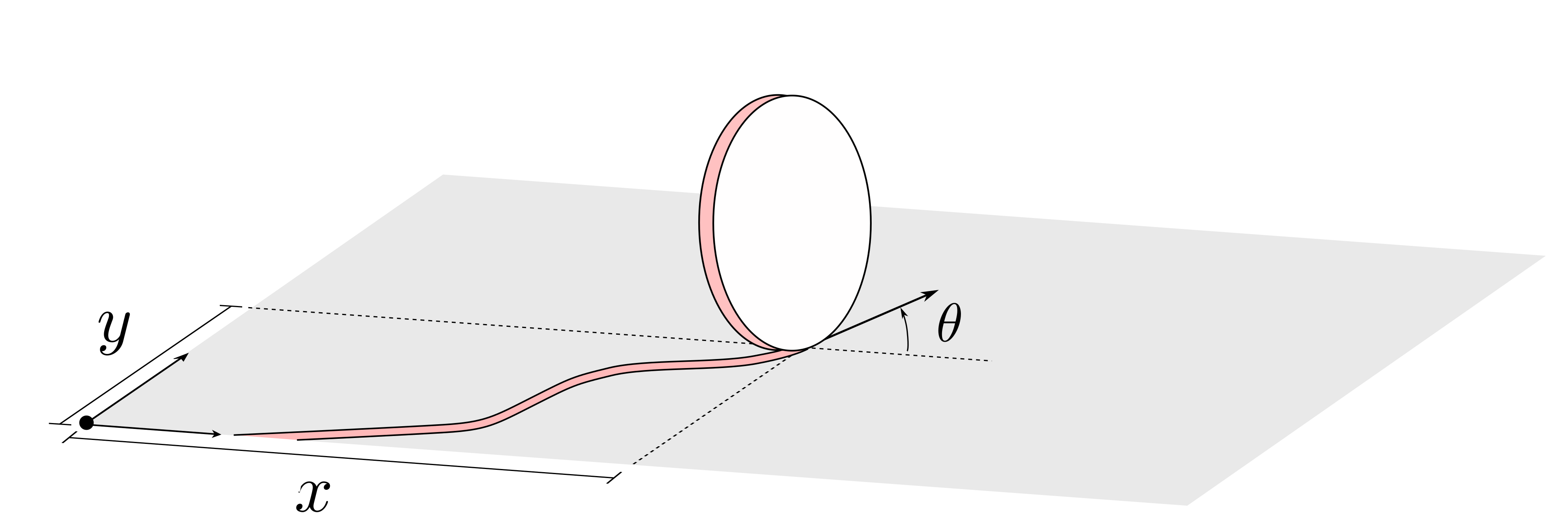
The configuration of a wheel rolling on a plane, as illustrated in Figure 1.1, can be represented by three parameters: the contact point position coordinates $\left(x,y\right)$ and the heading angle $\theta$ relative to a fixed reference frame. This set of parameters, $\bm{q}=\left[{x,y,\theta}\right]^{\top}$ , constitutes just one possible choice of generalized coordinates to define the wheel’s configuration. Alternatively, the configuration could also be represented using the heading angle $\theta$ along with a polar coordinate representation of the contact point position.

Refer to caption — Figure 1.1: Generalized coordinates for a wheel rolling without slipping on a plane.

1.2.2 Kinematic Constraints

Once a specific set of generalized coordinates, $\bm{q}$ , is chosen to represent a robot’s configuration, we can identify the relevant kinematic constraints for the robot. These kinematic constraints establish relationships between the generalized coordinates and the generalized velocities, thereby describing the limitations on the robot’s motion. We refer the reader to Siciliano et al. (2008)¹1. Siciliano, Bruno, Sciavicco, Lorenzo, Villani, Luigi, Oriolo, Giuseppe. Robotics: Modelling, Planning and Control. Springer Publishing Company, Incorporated, 2008. for a comprehensive treatment of robotic kinematics and the formulation of the associated constraint equations.

Definition 1.3 (Kinematic Constraints).

Kinematic constraints are a set of constraints imposed on the generalized coordinates, $\bm{q}$ , and generalized velocities, $\dot{\bm{q}}$ . We express kinematic constraints mathematically as:

\tilde{a}_{i}(\bm{q},\dot{\bm{q}})=0,\quad\quad i=1,\dots,k<n_{g},

(1.5)

where $k$ is the number of constraints and $n_{g}$ is the number of generalized coordinates.

In many robotics applications, kinematic constraints are linear with respect to the generalized velocities. These are known as Pfaffian constraints, and can be mathematically expressed as:

\bm{a}_{i}^{\top}(\bm{q})\dot{\bm{q}}=0,\quad\quad i=1,\dots,k<n_{g},

(1.6)

where $\bm{a}_{i}(\bm{q})\in\mathbb{R}^{n_{g}}$ . Pfaffian constraints can also be compactly represented in matrix form as:

A^{\top}(\bm{q})\dot{\bm{q}}=\bm{0},

(1.7)

where $A(\bm{q})\in\mathbb{R}^{n_{g}\times k}$ .

Example 1.2.2 (Pendulum).

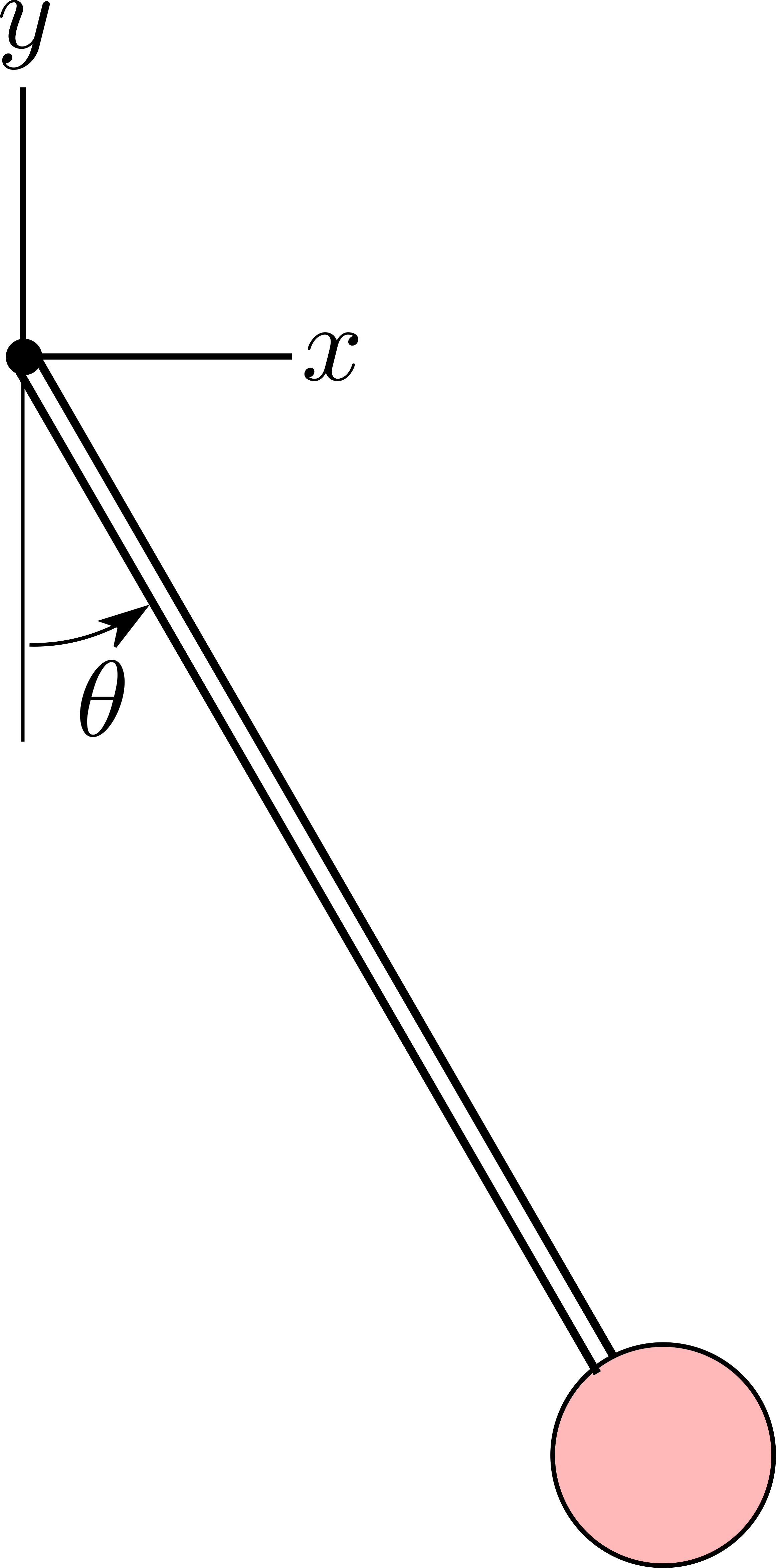
Figure 1.2 shows a simple pendulum with a point mass and a rigid, massless, rod that rotates about a fixed pivot point. We can choose to represent the configuration of the pendulum by the Cartesian coordinate position of the mass, assuming the pivot point is the reference frame origin. The generalized coordinate vector for this choice is $\bm{q}=\left[{x,y}\right]^{\top}$ , and the generalized velocity vector is $\dot{\bm{q}}=\left[{\dot{x},\dot{y}}\right]^{\top}$ . The fact that the rod connecting the pivot point to the mass is rigid introduces a restriction on the motion of this system, which we represent by the kinematic constraint:

\tilde{a}_{1}(\bm{q},\dot{\bm{q}})=x^{2}+y^{2}-L^{2}=0,

(1.8)

where $L$ is the length of the rod. While this constraint is not in Pfaffian form, we can equivalently express it as a Pfaffian constraint by noting that:

\tilde{a}_{1}(\bm{q},\dot{\bm{q}})=0\implies\frac{\partial\tilde{a}_{1}(\bm{q}% ,\dot{\bm{q}})}{\partial t}=0.

For the pendulum kinematic constraint in Equation 1.8, we have:

\frac{\partial\tilde{a}_{1}(\bm{q},\dot{\bm{q}})}{\partial t}=2x\dot{x}+2y\dot% {y},

and therefore we can write the constraint in the Pfaffian form of Equation 1.6 with:

\bm{a}_{i}^{\top}(\bm{q})=\begin{bmatrix}2x&2y\end{bmatrix}.

(1.9)

The Pfaffian constraint in Equation 1.9 implies that Equation 1.8 holds as long as the pendulum starts in a state $\bm{q}(0)$ satisfying $\tilde{a}_{1}(\bm{q}(0))=0$ .

An alternative choice of generalized coordinates to represent the pendulum’s configuration is to consider the angle $\theta$ between the vertical and the pendulum’s rod orientation, $\bm{q}=[\theta]$ . This choice fully specifies the configuration without requiring us to define any kinematic constraints, making it a more natural choice for this system. Note that since $x=L\sin\theta$ and $y=-L\cos\theta$ the kinematic constraint in Equation 1.8 is trivially satisfied for all $\theta$ .

Example 1.2.3 (Rolling Wheel).

Consider the wheel illustrated in Figure 1.1, which we can represent with the generalized coordinates $\bm{q}=\left[{x,y,\theta}\right]^{\top}$ . For this system, we can assume that the friction at the contact point between the wheel and the surface induces a no-slip condition. This no-slip condition is a constraint on the motion of the wheel that restricts the velocity component of the wheel in the lateral direction to always be zero. Since the unit vector $\bm{e}_{v}=\left[{\cos\theta,\>\sin\theta}\right]^{\top}$ describes the heading of the wheel, the lateral direction is given by the perpendicular unit vector $\bm{e}_{v,\perp}=\left[{\sin\theta,\>-\cos\theta}\right]^{\top}$ . We can compute the lateral velocity from the dot product of the lateral direction unit vector and the velocity vector, $\bm{v}=\left[{\dot{x},\>\dot{y}}\right]^{\top}$ , which gives the no-slip kinematic constraint:

a_{1}(\bm{q},\dot{\bm{q}})=\dot{x}\sin\theta-\dot{y}\cos\theta=0.

(1.10)

This constraint is linear in the generalized velocities, $\left(\dot{x},\dot{y}\right)$ , and therefore is a Pfaffian constraint.

1.2.3 Holonomic and Nonholonomic Constraints

Kinematic constraints often fall into two categories: holonomic or nonholonomic, depending on how they restrict the motion of the system. Holonomic constraints can be expressed solely as functions of the generalized coordinates, without involving generalized velocities. In contrast, nonholonomic constraints involve the generalized velocities and cannot be expressed solely in terms of the generalized coordinates.

Definition 1.4 (Holonomic Constraints).

Kinematic constraints that can be expressed in the form:

\tilde{a}_{i}(\bm{q})=0,\quad i=1,\dots,k<n_{g},

(1.11)

are called holonomic.

In robotics applications, holonomic constraints generally arise due to mechanical interconnections, such as rigid links and joints of a robotic arm. We refer to a system that is only subject to holonomic constraints as a holonomic system. These constraints are a unique subclass of kinematic constraints that restrict the accessible configurations of the system. Specifically, for a system with $n$ generalized coordinates under $k$ holonomic constraints, the dimension of the space of accessible configurations is $n-k$ . Holonomic constraints can always be equivalently expressed as Pfaffian constraints of the form Equation 1.6. This is because:

\tilde{a}_{i}(\bm{q})=0\implies\frac{\partial\tilde{a}_{i}(\bm{q})}{\partial t% }=0,

and by differentiating the expression:

\frac{\partial\tilde{a}_{i}(\bm{q})}{\partial t}=\frac{\partial\tilde{a}_{i}(% \bm{q})}{\partial\bm{q}}\dot{\bm{q}}=\bm{a}_{i}^{\top}(\bm{q})\dot{\bm{q}},

(1.12)

as we demonstrated in Example 1.2.2. However, it is important to note that not all Pfaffian constraints are holonomic. For a Pfaffian constraint to be holonomic, it must be integrable to the form in Equation 1.11. Specifically, there must exist a scalar function $\tilde{a}_{i}(\bm{q})$ such that:

\bm{a}_{i}^{\top}(\bm{q})\dot{\bm{q}}=\frac{\partial\tilde{a}_{i}(\bm{q})}{% \partial\bm{q}}\dot{\bm{q}}=0.

(1.13)

This implies that the Pfaffian constraint, when integrated, yields a constraint solely dependent on the generalized coordinates $\bm{q}$ , without any explicit dependence on their time derivatives $\dot{\bm{q}}$ .

Example 1.2.4 (Pendulum).

Consider the pendulum from Example 1.2.2. The kinematic constraint in Equation 1.8 restricts the pendulum mass to lie on a circle of radius $L$ , which is a subset of all possible generalized coordinates. This constraint is holonomic since we can express it as a function of only the generalized coordinates.

Example 1.2.5 (Rolling Wheel).

Consider the wheel from Example 1.2.3, where the kinematic constraint in Equation 1.10 restricts the direction of motion. In contrast to the pendulum, this constraint does not limit the wheel’s ability to reach any configuration of generalized coordinates, namely the position and heading. Mathematically, we cannot integrate the constraint in Equation 1.10 to yield a constraint of the form $\tilde{a}_{i}(\bm{q})=0$ , and thus this constraint is not holonomic.

While holonomic constraints restrict the system’s accessible configurations, kinematic constraints can also limit the motion between configurations. We refer to these constraints as nonholonomic constraints. A system that is subject to at least one nonholonomic constraint is referred to as a nonholonomic system.

Definition 1.5 (Nonholonomic Constraints).

Constraints that can be described in Pfaffian form, $\bm{a}_{i}(\bm{q})^{\top}\dot{\bm{q}}=0$ , but cannot be integrated to the form $\tilde{a}_{i}(\bm{q})=0$ are called nonholonomic.

That is, the Pfaffian expressions cannot be written as the total time derivative of any scalar function that depends only on the generalized coordinates. In other words, there exists no scalar function $\tilde{a}_{i}(\bm{q})$ such that $\frac{d}{dt}\tilde{a}_{i}(\bm{q})=\bm{a}_{i}(\bm{q})^{\top}\dot{\bm{q}}$ . Geometrically, nonholonomic constraints restrict the instantaneous generalized velocities to lie in the null space of $A(\bm{q})^{\top}$ , where $A(\bm{q})$ is the matrix whose rows are the vectors $\bm{a}_{i}(\bm{q})^{\top}$ corresponding to each nonholonomic constraint.

Example 1.2.6 (Rolling Wheel).

Consider the wheel example from Example 1.2.3, which has a nonholonomic constraint:

a_{1}(\bm{q})^{\top}\dot{\bm{q}}=\begin{bmatrix}\sin\theta&-\cos\theta&0\end{% bmatrix}\dot{\bm{q}}=0.

The null space of $a_{1}(\bm{q})^{\top}$ in this case is spanned by the vectors $[\cos\theta,\>\sin\theta,\>0]$ and $[0,\>0,\>1]$ , which suggests that all motion must be made up of a linear combination of these vectors. Intuitively, we expect this because $[\cos\theta,\>\sin\theta,\>0]$ is the rolling direction and $[0,\>0,\>1]$ is the axis the wheel rotates about.

In summary, holonomic constraints restrict a system’s motion by confining its configurations to lower-dimensional manifolds—specifically, level sets defined by scalar equations of the form $\tilde{a}_{i}(\bm{q})=0$ . For a system with $n$ generalized coordinates and $k$ independent holonomic constraints, the configuration space is effectively reduced to a manifold of dimension $n-k$ . This reduction reflects a true loss of accessibility in the configuration space: the system can only evolve along a restricted subset of configurations determined by the initial conditions and the constraint equations. In contrast, nonholonomic constraints act directly on the system’s instantaneous velocities, typically expressed in Pfaffian form as $A(\bm{q})^{\top}\dot{\bm{q}}=0$ , where $A(\bm{q})^{\top}$ is a full-rank matrix of dimension $k\times n$ . These constraints restrict the allowed directions of motion at each configuration by confining $\dot{\bm{q}}$ to lie in an $(n-k)$ -dimensional subspace. However, since nonholonomic constraints are not integrable, they do not reduce the dimensionality of the configuration space itself. That is, although motion is constrained at each instant, the system may still be able to reach any configuration in the configuration space through admissible trajectories that respect the velocity constraints. Thus, while holonomic constraints reduce the number of independent configuration variables and confine the system to a lower-dimensional subset of the configuration space, nonholonomic constraints preserve full accessibility of the configuration space but restrict how that space can be traversed.

1.2.4 Kinematic Models

Once we have chosen an appropriate set of generalized coordinates $\bm{q}$ and have identified the relevant kinematic constraints, we can convert the kinematic constraints into a state space model of the form in Equation 1.1, which we refer to as a kinematic model.

Definition 1.6 (Kinematic Model).

Given a generalized coordinate vector $\bm{q}\in\mathbb{R}^{n_{g}}$ , and $k$ Pfaffian constraints^†^†margin: These Pfaffian constraints can come from a combination of holonomic and non-holonomic constraints. , $A^{\top}(\bm{q})\dot{\bm{q}}=\bm{0}$ , a kinematic model is a state space model of the form:

\dot{\bm{q}}=G(\bm{q})\bm{u},

(1.14)

where $\bm{u}\in\mathbb{R}^{p}$ is the input and where the column space of $G(\bm{q})\in\mathbb{R}^{n_{g}\times n_{g}-k}$ spans the null space of $A^{\top}(\bm{q})$ .

Each input in $\bm{u}$ corresponds to one degree of freedom of the system, and for any initial condition $\bm{q}(0)$ and sequence of inputs $\bm{u}(t)$ the solutions to the kinematic model are guaranteed to satisfy the Pfaffian constraints. We can prove that the trajectories of the kinematic model will satisfy the Pfaffian constraints by writing the model in the equivalent form:

\dot{\bm{q}}=G(\bm{q})\bm{u}=\sum_{i=1}^{n-k}\bm{g}_{i}(\bm{q})u_{i},

where $\bm{g}_{i}\in\mathbb{R}^{n_{g}}$ is the $i$ -th column of $G$ and $u_{i}$ is the $i$ -th input. In this form, we can more easily see that each input acts on the generalized velocity $\dot{\bm{q}}$ through a particular mode that is defined by the vector $\bm{g}_{i}$ . Since we have specified in Definition 1.6 that the column space of $G$ spans the null space of $A^{\top}(\bm{q})$ , we know that by definition:

A^{\top}(\bm{q})\bm{g}_{i}(\bm{q})u_{i}=0,

for any input $u_{i}\in\mathbb{R}$ and for all coordinates $\bm{q}$ . Therefore, by definition each component of the input vector can only influence the generalized velocity in a way that satisfies the Pfaffian constraints. Another way to see this mathematically is by substituting the kinematic model into the Pfaffian constraint equation:

\begin{split}A^{\top}(\bm{q})\dot{\bm{q}}&=A^{\top}(\bm{q})G(\bm{q})\bm{u},\\ &=A^{\top}(\bm{q})\big{(}\sum_{i=1}^{n-k}\bm{g}_{i}(\bm{q})u_{i}\big{)},\\ &=\sum_{i=1}^{n-k}A^{\top}(\bm{q})\bm{g}_{i}(\bm{q})u_{i},\\ &=0.\\ \end{split}

Example 1.2.7 (Rolling Wheel).

Consider the rolling wheel example from Example 1.2.3, which has a single nonholonomic constraint:

a_{1}(\bm{q})^{\top}\dot{\bm{q}}=\begin{bmatrix}\sin\theta&-\cos\theta&0\end{% bmatrix}\dot{\bm{q}}=0,

where $\bm{q}=\left[{x,\>y,\>\theta}\right]^{\top}$ . The null space of $a_{1}(\bm{q})^{\top}$ is spanned by the vectors $\left[{\cos\theta,\>\sin\theta,\>0}\right]^{\top}$ and $\left[{0,\>0,\>1}\right]^{\top}$ and therefore the kinematic model is given by:

\begin{bmatrix}\dot{x}\\ \dot{y}\\ \dot{\theta}\end{bmatrix}=\begin{bmatrix}\cos\theta&0\\ \sin\theta&0\\ 0&1\end{bmatrix}\begin{bmatrix}u_{1}\\ u_{2}\end{bmatrix}.

(1.15)

In this case, the inputs $u_{1}$ and $u_{2}$ have an intuitive physical meaning: $u_{1}$ is the speed at which the wheel is moving, and $u_{2}$ is the wheel’s angular rotation rate.

1.2.5 Dynamics Models

Kinematic models describe the geometric constraints that limit a robot’s motion—for example, the fact that a robotic arm can only rotate about its joints. However, kinematics alone does not explain how motion is generated or resisted. For that, we turn to dynamics, which describe how forces and torques influence motion by producing accelerations.

Newton’s second law of motion is the foundation of robot dynamics, relating the net force acting on a body to its acceleration. Applied to a single point mass, the law takes the form:

\bm{F}(\bm{q},\dot{\bm{q}})=m\ddot{\bm{q}},

(1.16)

where $m$ is the mass of the particle, $\bm{q}=\left[{x,y,z}\right]^{\top}$ is its position vector, and $\bm{F}$ is the total force acting on the particle.

Example 1.2.8 (Mass-spring-damper system).

A fundamental example in the study of dynamics is the one-dimensional mass-spring-damper system. The system consists of a mass $m$ attached to a spring and a damper, constrained to move along a line. The total force acting on the mass is typically composed of three terms:

1.

an external input force $F_{\text{external}}$ ,
2.

a spring force $-kx$ that resists displacement from the equilibrium position, and
3.

a damping force $-c\dot{x}$ that resists velocity.

The net force on the mass is:

F=F_{\text{external}}-kx-c\dot{x},

where $k>0$ and $c>0$ are the spring and damping coefficients, respectively, and $x$ is the displacement from equilibrium. Substituting this expression into Newton’s second law yields the following second-order differential equation:

m\ddot{x}+c\dot{x}+kx=F_{\text{external}}.

This equation models oscillatory motion with damping, and it arises in many robotics applications—for example, when analyzing joint compliance, actuator dynamics, or contact interactions.

While the mass-spring-damper system illustrates the dynamics of a single particle in one dimension, real-world robotic systems are often more complex. To capture their behavior, we extend Newton’s second law to systems of interconnected particles, typically modeled in robotics as rigid bodies. A rigid body is an idealized object in which the relative positions of all constituent particles remain fixed over time, regardless of external forces. This assumption implies that the body does not deform and allows us to reduce a complex system of interacting particles to a simpler model governed by the motion of a finite set of parameters, for example, position and orientation of a frame fixed to the body. As a result, rigid body dynamics provide a powerful and tractable framework for analyzing and simulating robotic systems^†^†margin: Interesting examples in robotics where the rigid body assumption may not hold include soft robots, robots with compliant end-effectors, or robots with lightweight flexible structures. .

The motion of a rigid body in three-dimensional space can be described in terms of its translational and rotational dynamics. Translational dynamics govern the motion of the body’s center of mass and are described by Newton’s second law, as expressed in Equation 1.16, where the position variable refers specifically to the center of mass. In three-dimensional space, a rigid body has three translational degrees of freedom, corresponding to movement along each of the Cartesian axes. Rotational dynamics, on the other hand, describe how the body’s orientation evolves over time. A rigid body also has three degrees of freedom associated with its orientation in three-dimensional space, corresponding to rotation about each of its principal axes. Unlike translation, orientation cannot be represented by a single vector, and several parameterizations are commonly used. Notable examples include rotation matrices, which provide a full and unambiguous representation at the cost of redundancy; Euler angles, which use a sequence of three rotations to represent orientation, and quaternions, which offer a compact and singularity-free alternative well-suited for numerical applications.

The rotational dynamics^†^†margin: We refer the reader to Shuster (1993)²2. Shuster, M. D. “Survey of attitude representations.” Journal of the Astronautical Sciences 41(4), 439-517, 1993. for an in-depth treatment of rotational dynamics and attitude representations. of a rigid body are governed by the time evolution of its angular momentum. Specifically, they are described by:

\bm{M}=\dot{\bm{H}},

(1.17)

where $\bm{M}$ denotes the total external moment (or torque) acting on the body, and $\bm{H}$ is the angular momentum, typically computed about the center of mass. This relationship is commonly referred to as Euler’s equation for rotational dynamics and captures how applied torques influence changes in the body’s rotational motion.

An alternative to the Newton-Euler method—defined by Equations (Equation 1.16)-(Equation 1.17)—for deriving the equations of motion for a rigid body is the Lagrange Method. This approach is closely tied to the notion of generalized coordinates, generalized velocities, and kinematic constraints, and takes an energy-based approach. In the Lagrange method, the dynamics of a rigid body are derived from a scalar quantity called the Lagrangian, defined as the difference between the kinetic and potential energies:

L(\bm{q},\dot{\bm{q}})=T(\bm{q},\dot{\bm{q}})-V(\bm{q}),

(1.18)

where $T(\bm{q},\dot{\bm{q}})$ and $V(\bm{q})$ denote the kinetic and potential energies of the system, respectively. The evolution of the system is governed by Lagrange’s equations ⁵5. Siciliano, B., Sciavicco, L., Villani, L., Oriolo, G. Robotics: Modelling, Planning and Control. Springer Publishing Company, Incorporated, 2008.⁶6. Lynch, K. M., Park, K. C. Modern Robotics: Mechanics, Planning, and Control. Cambridge University Press, 2017., which incorporate both external influences and kinematic constraints. In the absence of constraints, the equations of motion are given by:

\begin{split}\frac{d}{dt}\Big{(}\frac{\partial L}{\partial\dot{\bm{q}}_{j}}% \Big{)}-\frac{\partial L}{\partial\bm{q}_{j}}=Q_{j},\quad j=1,\dots,n_{g},\end% {split}

(1.19)

where $Q_{j}\in\mathbb{R}$ is a non-conservative generalized force associated with the generalized coordinate $\bm{q}_{j}$ ^†^†margin: Generalized forces are projections of physical forces and torques into the generalized coordinate space. Forces not derived from a potential—such as friction—are termed non-conservative. In contrast, forces like gravity are conservative. , and $n_{g}$ corresponds to the system’s degrees of freedom. Equations (Equation 1.19) describe how the generalized forces acting on the system relate to its position, velocity, and acceleration, providing a systematic way to derive the system’s dynamic model from its kinetic and potential energies.

In the presence of Pfaffian constraints^†^†margin: While Lagrange’s method can accommodate general constraints, we focus here on Pfaffian constraints for simplicity. , Lagrange’s equations take the form:

\begin{split}\frac{d}{dt}\Big{(}\frac{\partial L}{\partial\dot{\bm{q}}_{j}}% \Big{)}-\frac{\partial L}{\partial\bm{q}_{j}}=Q_{j}+\sum_{i=1}^{k}\lambda_{i}a% _{ij}(\bm{q}),\quad j=1,\dots,n_{g},\\ \bm{a}_{i}^{\top}(\bm{q})\dot{\bm{q}}=0,\quad\quad i=1,\dots,k,\end{split}

(1.20)

where $a_{ij}$ is the $j$ -th component of the $i$ -th Pfaffian constraint vector $\bm{a}_{i}(\bm{q})$ and $\lambda_{i}\in\mathbb{R}$ is a Lagrange multiplier. The first $n_{g}$ equations describe the dynamics of the generalized coordinates under the influence of both external and constraint forces, while the remaining $k$ equations represent the kinematic constraints themselves. The complete system thus comprises $n_{g}+k$ equations in $n_{g}+k$ unknowns (the generalized coordinates and the Lagrange multipliers), and is commonly referred to as the standard non-holonomic form. If the system is holonomic and the generalized coordinates are chosen to be independent, the constraints are implicitly satisfied, and Lagrange’s equations reduce to the simpler, unconstrained form introduced in Equation 1.19.

Example 1.2.9 (Pendulum).

Consider again the pendulum depicted in Figure 1.2. To model its dynamics, we analyze how gravity drives the motion of the mass. Specifically, we will demonstrate four distinct approaches for deriving the equations of motion—using both Cartesian and polar coordinates, and applying both the Newton-Euler and Lagrange methods. This comparison will highlight how the choice of generalized coordinates can influence the complexity of the derivation.

We begin by using Newton’s second law to derive the dynamics of the pendulum, focusing on the two forces acting on the mass: gravity and the force from the rod. We assume that the rod’s force acts purely along its axis. Since the pendulum’s length is fixed, this force must counteract the component of gravity along the rod and generate the required centripetal acceleration. The axial force exerted by the rod is given by:

F_{r}=mg\cos\theta+\frac{mv^{2}}{L},

where $m$ is the mass of the pendulum, $g$ is gravitational acceleration, $L$ is the length of the rod, and $v$ is the speed of the mass. The gravitational force is:

F_{g}=mg,

acting along the negative $y$ -direction. To compute the net force in Cartesian coordinates, we project both the rod’s force and the gravitational force onto the $x$ - and $y$ -axes:

\begin{split}F_{x}&=-\frac{mv^{2}}{L}\sin\theta-mg\sin\theta\cos\theta,\\ F_{y}&=\frac{mv^{2}}{L}\cos\theta-mg\sin^{2}\theta.\end{split}

Applying Newton’s second law as defined in Equation 1.16 yields the equations of motion:

\begin{split}\ddot{x}&=-\frac{v^{2}}{L}\sin\theta-g\sin\theta\cos\theta,\\ \ddot{y}&=\frac{v^{2}}{L}\cos\theta-g\sin^{2}\theta.\end{split}

To express these equations purely in terms of Cartesian coordinates, we substitute $x=L\sin\theta$ and $y=-L\cos\theta$ , leading to:

\begin{split}\ddot{x}&=\frac{1}{L^{2}}(gxy-xv^{2}),\\ \ddot{y}&=-\frac{1}{L^{2}}(gx^{2}+yv^{2}),\end{split}

(1.21)

with $v^{2}=\dot{x}^{2}+\dot{y}^{2}$ . This method requires careful force analysis, as the kinematic constraint (fixed-length rod) is handled implicitly through the projected components of the rod’s force.

As a second approach to deriving the equations of motion using Cartesian coordinates, we now apply the Lagrange method, which yields a slightly simpler formulation. We begin by defining the kinetic and potential energies:

T=\frac{1}{2}m(\dot{x}^{2}+\dot{y}^{2}),\quad V=mgy,

and observe that there are no external non-conservative generalized forces^†^†margin: Gravity is a conservative force, so no generalized non-conservative forces appear. . As discussed in Example 1.2.2, we recall the system’s single Pfaffian constraint:

x\dot{x}+y\dot{y}=0.

Thus, using Lagrange’s equations introduced in Equation 1.20, we obtain:

\begin{split}m\ddot{x}&=\lambda x,\\ m\ddot{y}+mg&=\lambda y,\\ x\dot{x}+y\dot{y}&=0.\end{split}

(1.22)

We can solve for the Lagrange multiplier $\lambda$ by differentiating the constraint with respect to time:

\frac{d}{dt}(x\dot{x}+y\dot{y})=\dot{x}^{2}+\dot{y}^{2}+x\ddot{x}+y\ddot{y}=0,

and by substituting the expressions for $\ddot{x}$ and $\ddot{y}$ from the first two Lagrange’s equations in (Equation 1.22) to obtain:

\dot{x}^{2}+\dot{y}^{2}+\frac{1}{m}x^{2}\lambda+\frac{1}{m}y^{2}\lambda-gy=0.

Solving for $\lambda$ yields:

\lambda=\frac{m}{L^{2}}(gy-v^{2}),

where we used $L^{2}=x^{2}+y^{2}$ and $v^{2}=\dot{x}^{2}+\dot{y}^{2}$ . Finally, substituting the expression for $\lambda$ back into the equations of motion and simplifying, we find:

\begin{split}\ddot{x}&=\frac{1}{L^{2}}(gxy-xv^{2}),\\ \ddot{y}&=-\frac{1}{L^{2}}(gx^{2}+yv^{2}),\\ \end{split}

(1.23)

which matches the result previously obtained using Newton’s method in Equation 1.21.

After applying both the Newton-Euler and Lagrange methods in Cartesian coordinates, we now replicate the derivation in polar coordinates. To apply Euler’s equation for rotational dynamics as given in Equation 1.17, we adopt a coordinate frame fixed at the pivot point. The gravitational force acting on the mass generates a moment about the pivot:

M=-mgL\sin\theta,

while the angular momentum of the system about the same point is:

H=mL^{2}\dot{\theta},

where $mL^{2}$ is the moment of inertia^†^†margin: In Euler’s equation, the moment of inertia plays a role analogous to mass in Newton’s second law. about the pivot. Substituting into Euler’s equation yields the system dynamics:

\ddot{\theta}=-\frac{g}{L}\sin\theta,

(1.24)

which are considerably more compact than the corresponding equations derived in Cartesian coordinates.

The Lagrange method also becomes significantly simpler when using the polar coordinate $\theta$ , as there is no need to handle Pfaffian constraints explicitly. In this formulation, the kinetic and potential energies of the system are:

T=\frac{1}{2}mL^{2}\dot{\theta}^{2},\quad V=-mgL\cos\theta.

Applying Equation 1.20, and noting the absence of non-conservative generalized forces or constraints, we obtain the following equation of motion:

\begin{split}\ddot{\theta}=-\frac{g}{L}\sin\theta,\end{split}

(1.25)

which, as expected, matches the result derived using Euler’s equation in Equation 1.24.

1.3 Wheeled Robot Motion Models

Robots are developed in diverse forms, sizes, and configurations, each featuring distinct mobility solutions tailored to specific applications. Among these, wheeled robots are particularly common because of their excellent mobility and simple design. In this section, we demonstrate how the concepts from the preceding sections can be applied to two classic and widely used motion models for simple wheeled robots: the unicycle model and the differential drive model.

1.3.1 Unicycle Model

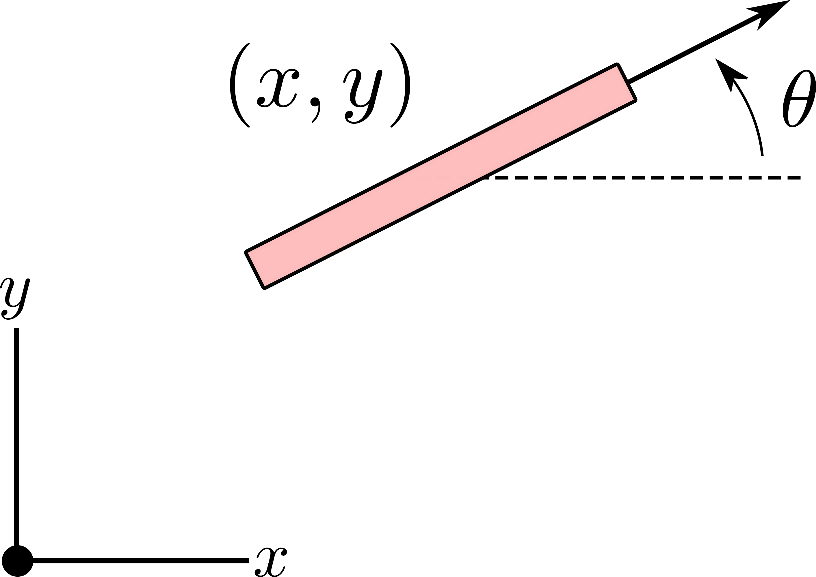
The unicycle model is one of the simplest kinematic models used for modeling robot motion. This model leverages the kinematics of the rolling wheel discussed in Example 1.2.3, essentially assuming the robot is constrained only by a no-slip constraint from a single wheel. Figure 1.3 illustrates a simplified diagram of the generalized coordinates for the unicycle model.

The kinematic model is identical to the one presented in Equation 1.15, namely:

\begin{bmatrix}\dot{x}\\ \dot{y}\\ \dot{\theta}\end{bmatrix}=\begin{bmatrix}\cos\theta&0\\ \sin\theta&0\\ 0&1\end{bmatrix}\begin{bmatrix}v\\ \omega\end{bmatrix},

(1.26)

where $v$ represents the forward speed and $\omega$ denotes the rotational rate.

While the unicycle model may be a simplified representation of the robot’s true kinematics, it remains valuable in many contexts where detailed dynamics are unnecessary. Its main advantage lies in its simplicity, which often enables more computationally efficient algorithms. In practice, such lower-fidelity models are often used in the early stages of a system’s design or decision-making process, and are later refined or supplemented with more accurate models when higher precision is required.

1.3.2 Differential Drive Model

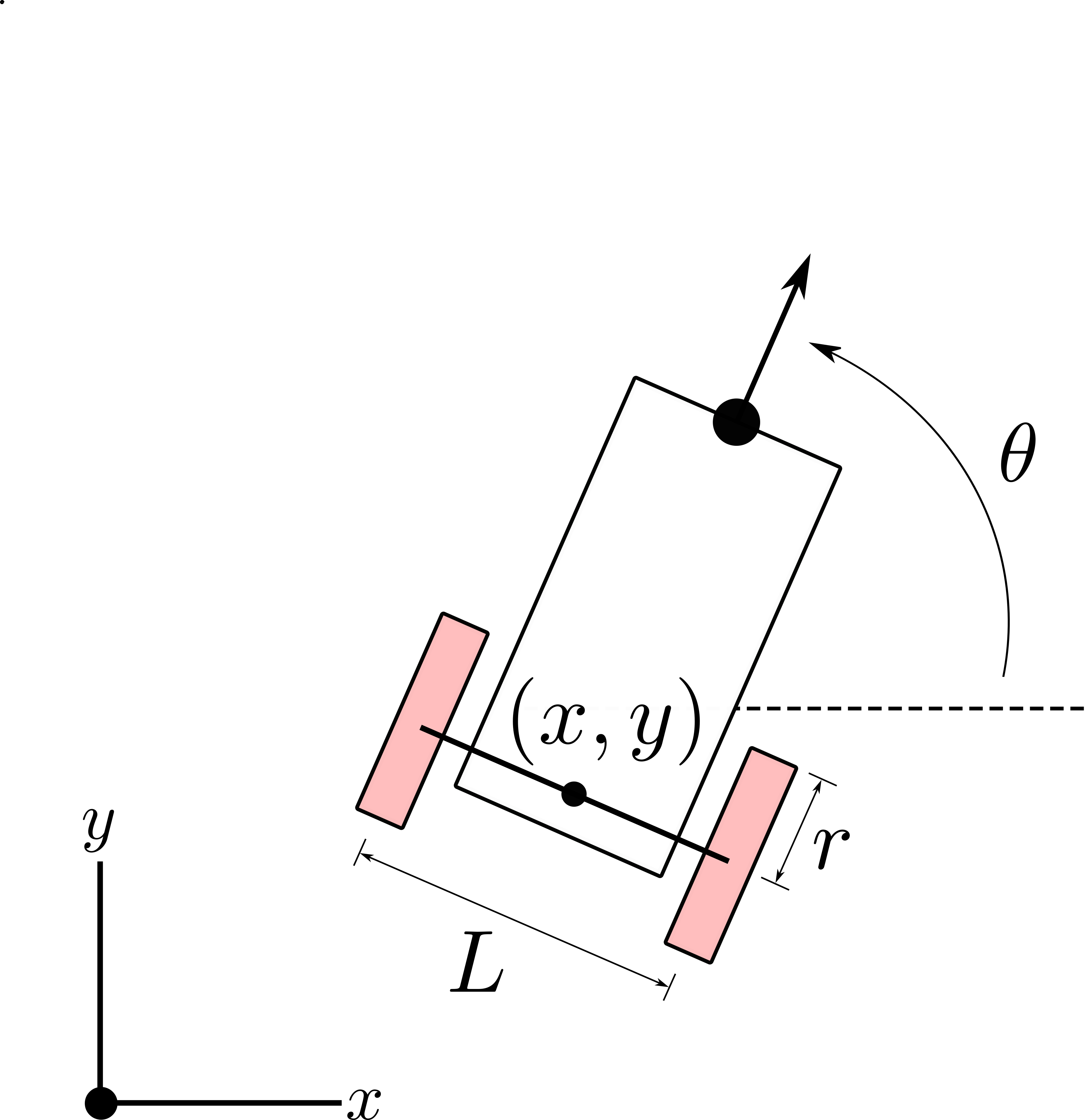
The differential drive model is a variation on the unicycle model from the previous section, with two wheels fixed on a shared rear axle and a passive front wheel that induces no additional kinematic constraints. This model uses the same generalized coordinates as the unicycle model, $\bm{q}=\left[{x,\>y,\>\theta}\right]^{\top}$ , but also requires the definition of certain geometric parameters: the width of the rear axle, denoted by $L$ , and the radius of the wheels, denoted by $r$ , as illustrated in Figure 1.4.

The differential drive model assumes the wheels roll without slipping, making the derivation of its kinematic constraints similar to that of a single rolling wheel, as discussed in Example 1.2.3. The heading vector of each wheel is given by $\bm{e}_{v}=\left[{\cos\theta,\>\sin\theta}\right]^{\top}$ , and the lateral direction is $\bm{e}_{v,\perp}=\left[{\sin\theta,\>-\cos\theta}\right]^{\top}$ . Using the lateral direction vector, we define the no-slip kinematic constraints for the wheels as:

\dot{\bm{p}}_{l}^{\top}\bm{e}_{v,\perp}=0,\quad\dot{\bm{p}}_{r}^{\top}\bm{e}_{% v,\perp}=0,

where $\dot{\bm{p}}_{l}$ and $\dot{\bm{p}}_{r}$ are the velocity vectors of the left and right wheels, respectively. Next, we express the wheel velocity vectors $\dot{p}_{l}$ and $\dot{p}_{r}$ as functions of the generalized coordinates and velocities by leveraging the robot’s geometry. The positions of the left and right wheel centers, denoted as $\bm{p}_{l}$ and $\bm{p}_{r}$ , respectively, can be computed from the generalized coordinates by:

\begin{split}\bm{p}_{l}=\begin{bmatrix}x-\frac{L}{2}\sin\theta\\ y+\frac{L}{2}\cos\theta\end{bmatrix},\quad\bm{p}_{r}=\begin{bmatrix}x+\frac{L}% {2}\sin\theta\\ y-\frac{L}{2}\cos\theta\end{bmatrix}.\end{split}

Taking the time derivative of these positions yields the velocity vectors:

\begin{split}\dot{\bm{p}}_{l}=\begin{bmatrix}\dot{x}-\dot{\theta}\frac{L}{2}% \cos\theta\\ \dot{y}-\dot{\theta}\frac{L}{2}\sin\theta\end{bmatrix},\quad\dot{\bm{p}}_{r}=% \begin{bmatrix}\dot{x}+\dot{\theta}\frac{L}{2}\cos\theta\\ \dot{y}+\dot{\theta}\frac{L}{2}\sin\theta\end{bmatrix}.\end{split}

After some algebraic manipulation, we find that the no-slip kinematic constraints for each wheel are equivalent:

\begin{split}\dot{\bm{p}}_{l}^{\top}\bm{e}_{v,\perp}&=\dot{\bm{p}}_{r}^{\top}% \bm{e}_{v,\perp}=\dot{x}\sin\theta-\dot{y}\cos\theta=0,\end{split}

indicating that the no-slip constraint for both wheels is redundant, and thus the constraint matches the single wheel constraint from Example 1.2.3. This is intuitive because the wheels are rigidly connected; hence, if one wheel cannot move laterally, neither can the other. The kinematic model for the differential drive model is also identical to the single wheel model in Equation 1.26, but the inputs can now be expressed in a more realistic form relative to the actual geometry of the robot.

In particular, instead of using the forward speed $v$ and body rotation rate $\omega$ as inputs, as in Equation 1.26, the differential drive model uses the rotation rates of the left and right wheels, $\omega_{l}$ and $\omega_{r}$ . We can derive a relationship between these sets of inputs by considering the geometry of the robot and the no-slip wheel assumption. First, denote the position $\bm{p}=\left[{x,\>y}\right]^{\top}$ in terms of the wheel center positions by $\bm{p}=\frac{1}{2}(\bm{p}_{l}+\bm{p}_{r})$ , thus the velocity vector is $\dot{\bm{p}}=\frac{1}{2}(\dot{\bm{p}}_{l}+\dot{\bm{p}}_{r})$ . By the no-slip wheel assumption, the velocity $v$ can be expressed as $v=\bm{e}_{v}^{\top}\dot{p}$ , leading to:

\begin{split}v&=\bm{e}_{v}^{\top}\dot{\bm{p}},\\ &=\frac{1}{2}\bm{e}_{v}^{\top}(\dot{\bm{p}}_{l}+\dot{\bm{p}}_{r}),\\ &=\frac{1}{2}(v_{l}+v_{r}),\\ &=\frac{r}{2}(\omega_{l}+\omega_{r}),\\ \end{split}

where $r$ is the radius of the wheel and $v_{l}$ and $v_{r}$ are the speeds of the left and right wheels, respectively. Additionally, the no-slip condition on each wheel is given by $v_{l}=\bm{e}_{v}^{\top}\dot{\bm{p}}_{l}$ and $v_{r}=\bm{e}_{v}^{\top}\dot{\bm{p}}_{r}$ , expanded as:

\begin{split}\dot{x}\cos{\theta}+\dot{y}\sin{\theta}-\dot{\theta}\frac{L}{2}&=% v_{l},\\ \dot{x}\cos{\theta}+\dot{y}\sin{\theta}+\dot{\theta}\frac{L}{2}&=v_{r}.\\ \end{split}

Since $\dot{x}\cos{\theta}+\dot{y}\sin{\theta}=v$ , we simplify these expressions to:

\begin{split}\frac{L}{2}\dot{\theta}&=v_{r}-v,\\ \frac{L}{2}\dot{\theta}&=v-v_{l}.\\ \end{split}

Combining these gives:

\begin{split}L\dot{\theta}&=v_{r}-v_{l},\\ &=r(\omega_{r}-\omega_{l}),\\ \end{split}

establishing the relationship between the generalized velocity $\dot{\theta}$ and the wheel rotational speeds.

In summary, the mapping between the inputs can be defined as:

v=\frac{r}{2}(\omega_{l}+\omega_{r}),\quad\omega=\frac{r}{L}(\omega_{r}-\omega% _{l}).

which allows us to define the differential drive model:

\begin{bmatrix}\dot{x}\\ \dot{y}\\ \dot{\theta}\end{bmatrix}=\begin{bmatrix}\frac{r}{2}\cos\theta&\frac{r}{2}\cos% \theta\\ \frac{r}{2}\sin\theta&\frac{r}{2}\sin\theta\\ \frac{r}{L}&-\frac{r}{L}\end{bmatrix}\begin{bmatrix}\omega_{r}\\ \omega_{l}\end{bmatrix}.

(1.27)

Despite the slight increase in complexity over the unicycle model, this model leverages the geometry of the robot to make the inputs more intuitive. This enhancement makes the differential drive model more suitable for certain motion planning and control tasks, as the robot’s actuation typically originates from motors attached to the wheels’ axles.

More generally, a kinematic state-space model should be interpreted only as a subsystem of a more comprehensive dynamical model. In particular, kinematic models typically assume direct control over certain motion variables—such as velocity or angular rate—without accounting for how these quantities are generated or constrained by the physical system. For more realistic modeling, it is often necessary to extend the kinematic model to include additional integrators in front of the control inputs.

Example 1.3.1 (Dynamic extension of the unicycle model).

The unicycle model introduced in Equation 1.26 assumes direct control over the forward velocity $v$ and angular velocity $\omega$ , with the state defined by the variables $\left(x,y,\theta\right)$ . To reflect the fact that velocity $v$ is itself the result of integrating an acceleration input $a$ , the model can be extended by treating $v$ as an additional state, yielding the augmented state $\left(x,y,\theta,v\right)$ and input $\left(\omega,a\right)$ . The dynamics become:

\begin{bmatrix}\dot{x}\\ \dot{y}\\ \dot{\theta}\\ \dot{v}\end{bmatrix}=\begin{bmatrix}v\cos\theta\\ v\sin\theta\\ \omega\\ a\end{bmatrix}.

(1.28)

This dynamic extension accounts for acceleration as a control input and enables the modeling of more realistic scenarios, such as those involving actuation limits.

1.3.3 Bicycle/Simple Car Model

The bicycle model is a simplified kinematic model commonly used to approximate the motion of vehicles with two front-steered wheels and two rear-driven wheels, such as cars or mobile robots with similar geometry. The model captures key steering dynamics while assuming no slip at the contact points of the wheels. It is called a “bicycle” model because the two front wheels and two rear wheels are collapsed into a single front and rear wheel aligned on a common axis, forming a virtual two-wheeled vehicle. Compared to the unicycle and differential drive models introduced earlier, the bicycle model enforces more realistic kinematic constraints on how the system can turn. In particular, it captures the fact that the vehicle must steer to follow curved paths, and cannot rotate in place. As such, it provides a better approximation for many wheeled systems while still remaining relatively simple.

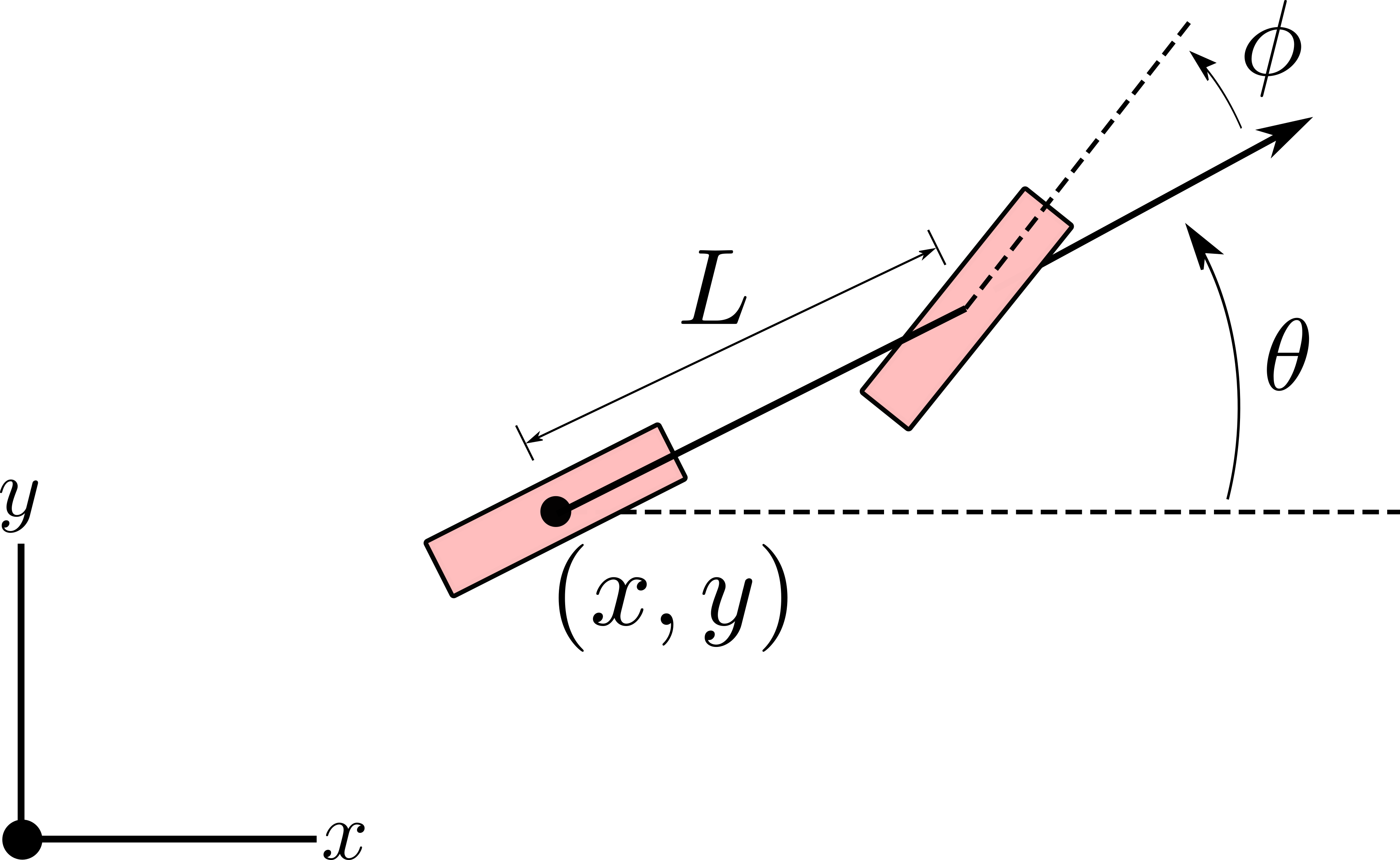
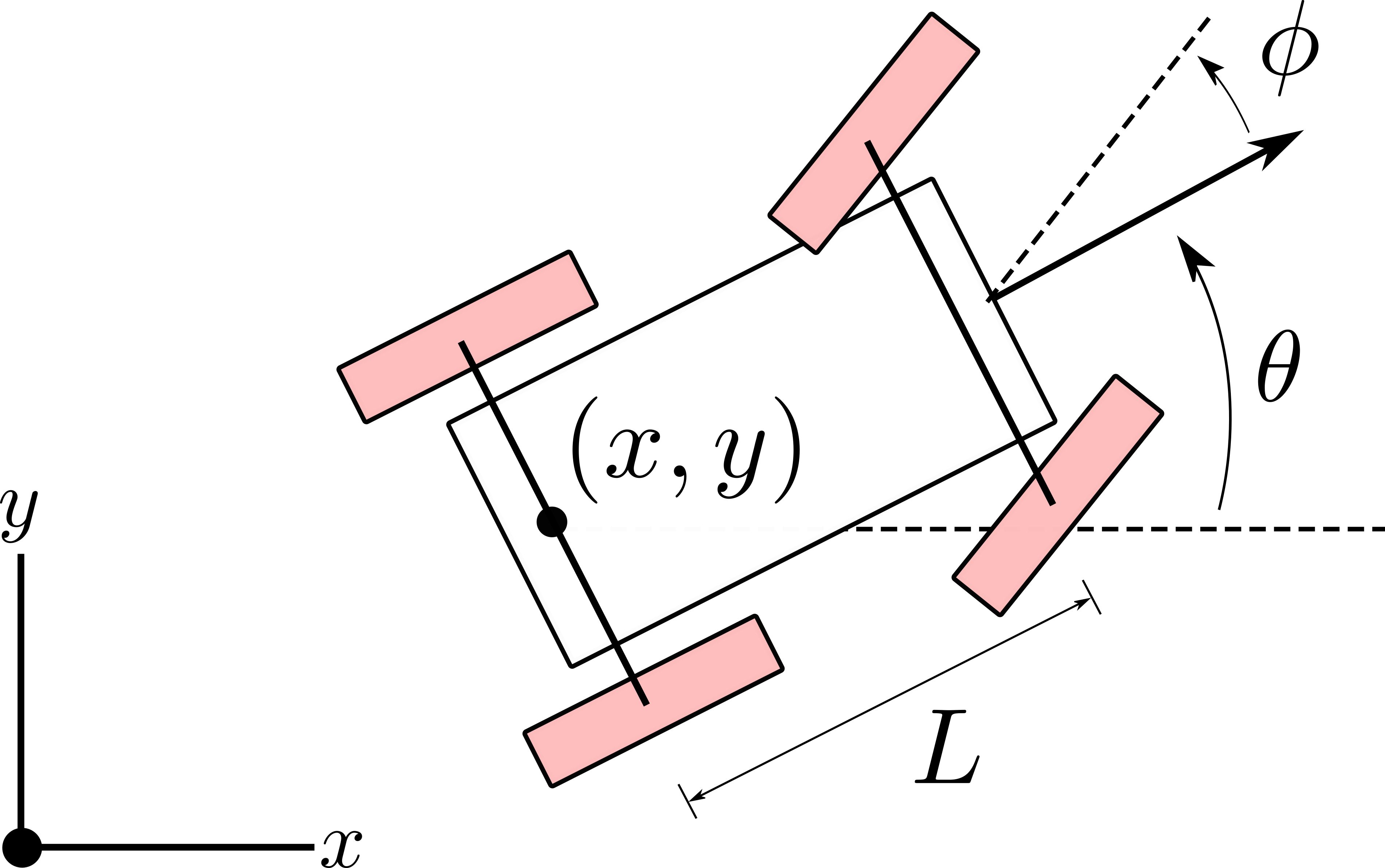
Figure 1.5 shows the simplified geometry of the bicycle model. This model can be derived by enforcing nonholonomic constraints on the rolling direction of each wheel and assuming ideal no-slip contact, following the discussion in previous sections. Figure 1.6 illustrates how the same kinematic model can be interpreted in the context of a four-wheeled vehicle. The key idea is that both front wheels steer with a common angle $\phi$ , and the vehicle moves forward with velocity $v$ , subject to the no-slip constraints. These assumptions lead to the following differential equations characterizing the car model:

\begin{split}\dot{x}&=v\cos\theta,\\ \dot{y}&=v\sin\theta,\\ \dot{\theta}&=\frac{v}{L}\tan\phi,\end{split}

(1.29)

where $\left(x,y\right)$ is the position of the rear axle center, $\theta$ is the heading angle, $v$ is the forward speed, $\phi$ is the steering angle, and $L$ is the length of the wheelbase (the distance between the front and rear axles). Therefore, we define the state as $\bm{x}=\left[{x,\>y,\>\theta}\right]^{\top}$ and the control input as $\bm{u}=\left[{v,\>\phi}\right]^{\top}$ .

1.4 Simulating Robot Dynamics

In Section 1.1, we introduced the concept of a state space model to mathematically describe the evolution of a robot’s state over time. In Section 1.2 we demonstrated how a robot’s kinematics and dynamics are used to derive a state space model that represents its physical motion. In this section, we present several computational techniques for simulating the changes in a robot’s state over time.

The state space model in Equation 1.1 is a general system of ordinary differential equations, which in most cases cannot be solved analytically. Numerical simulation provides a practical approach to obtaining approximate solutions, allowing us to better understand a robot’s dynamics and to test and validate algorithms for robot autonomy. Typically, when we refer to simulating a system, we mean approximately solving an initial value problem (IVP) for a system of differential equations, as defined in Equation 1.1:

\dot{\bm{x}}=h(\bm{x}(t),t),\quad\bm{x}(t_{0})=\bm{x}_{0},

where $h(\bm{x}(t),t)=f(\bm{x}(t),\bm{u}(t))$ , and the input $\bm{u}(t)$ may either be explicitly defined as a known function of time (e.g., a predefined control sequence), or computed at each time step based on the current state.

The objective of this initial value problem is to find the trajectory $\bm{x}(t)$ , starting from $\bm{x}(t_{0})$ , that satisfies the differential equation^†^†margin: If $h$ is Lipschitz continuous in $x(t)$ and continuous in $t$ , the trajectory $x(t)$ exists and is unique. . By the Fundamental Theorem of Calculus^†^†margin: This expresses the inverse relationship between differentiation and integration: integrating the derivative $\dot{\bm{x}}=h(\bm{x}(t),t)$ over time recovers the original function $\bm{x}(t)$ . , the solution at time $t$ can be written as:

\begin{split}\bm{x}(t)&=\bm{x}(t_{0})+\int_{t_{0}}^{t}h(\bm{x}(\tau),\tau)d% \tau.\end{split}

In general, evaluating this integral analytically for arbitrary functions $h(\bm{x}(t),t)$ is intractable. Therefore, we typically resort to numerical integration methods that involve a discretization in time:

\begin{split}\bm{x}(t)&=\bm{x}(t_{0})+\sum_{k=0}^{N-1}\int_{t_{k}}^{t_{k+1}}h(% \bm{x}(\tau),\tau)d\tau,\end{split}

(1.30)

where $t_{0}<t_{1}<\dots<t_{N}=t$ define a time grid, and each interval has width $\Delta t_{k}=t_{k+1}-t_{k}$ . This decomposition breaks the continuous integration problem into a sum of smaller integrals over short intervals. Within each interval $[t_{k},t_{k+1}]$ , we can then approximate the integral using various numerical quadrature rules—such as the Euler method, the Midpoint method, or higher-order Runge-Kutta schemes—which trade off computational cost and accuracy. In this section, we provide a concise introduction to some of the most widely used methods.

Example 1.4.1 (Simple IVP).

To illustrate the different numerical integration methods, we will consider the initial value problem defined below and presented in Algorithm 1.1 as an example:

\dot{x}(t)=x(t)\sin^{2}(t),\quad x(0)=1.

Our goal is to approximate the trajectory $x(t)$ over the interval $[0,10]$ using various integration methods.

⬇

import numpy as np

# Define the derivative function h(x, t)

def h(x, t):

return x * np.sin(t) ** 2

# Define initial conditions and final time

x0 = 1.0 # Initial state x(t0)

t0 = 0.0 # Initial time t0

tf = 10.0 # Final time tf

\Delta

t = 0.5 # Discretization step

t = np.arange(t0, tf +

\Delta

\Delta

t) # Array of timestamps

# Compute analytical solution

x_true = x0*np.exp(((t-t0) - np.sin(t-t0)*np.cos(t+t0))/2)

def integrate(h, x0, t, method):

x = np.zeros((t.size, x0.size))

x[0] = x0

for i in range(t.size - 1):

\Delta

t = t[i + 1] - t[i]

x[i + 1] = method(h, x[i], t[i],

\Delta

return x

def method(h, x, t,

\Delta

t):

# Implement here numerical integration method

# Test a specific numerical method

x_method = integrate(h, x0, t, method)

Algorithm 1.1: Definition of an illustrative initial value problem. The code for this example is available in the repository github.com/StanfordASL/pora-exercises in the notebook ch01/simulation.ipynb. In the following sections, we will explore different numerical integration methods and implement them in a custom method function.

Concretely, we will explore different techniques to approximate the following analytical solution:

x(t)=x_{0}\exp\left(\frac{t-t_{0}-\sin(t-t_{0})\cos(t+t_{0})}{2}\right),

which, for our specific initial conditions $x_{0}=1$ and $t_{0}=0$ , simplifies to:

x(t)=\exp\left(\frac{t-\sin(t)\cos(t)}{2}\right).

1.4.1 Euler Method

One of the simplest techniques for approximating the integral within each time interval of the discretized problem, as shown in Equation 1.30, is the Euler method^†^†margin: Named after the Swiss mathematician Leonhard Euler and often referred to as the forward Euler method. . This method approximates the integral over a short interval $[t_{k},t_{k+1}]$ by evaluating the integrand at the beginning of the interval.

Given that the trajectory $\bm{x}(t)$ satisfies:

\bm{x}(t_{k+1})=\bm{x}(t_{k})+\int_{t_{k}}^{t_{k+1}}h(\bm{x}(\tau),\tau)d\tau,

the Euler method approximates this integral by assuming $h(\bm{x}(\tau),\tau)$ is constant within the interval, yielding:

\bm{x}(t_{k+1})\approx\bm{x}(t_{k})+\Delta t\cdot h(\bm{x}(t_{k}),t_{k}),

where $\Delta t=t_{k+1}-t_{k}$ is the time step.

This approximation corresponds to a first-order Taylor series expansion:

\begin{split}\bm{x}(t+\Delta t)&\approx\bm{x}(t)+\Delta t\,\dot{\bm{x}}(t),\\ &=\bm{x}(t)+\Delta t\cdot h(\bm{x}(t),t),\\ \end{split}

(1.31)

which treats the rate of change $\dot{\bm{x}}(t)$ as constant across the interval.

Alternatively, the Euler method can be interpreted as a finite difference approximation of the time derivative:

\dot{\bm{x}}(t)\approx\frac{\bm{x}(t+\Delta t)-\bm{x}(t)}{\Delta t}.

While computationally inexpensive, the Euler method has limited accuracy due to its reliance on information from the beginning of each interval. The local truncation error^†^†margin: That is, the error introduced in a single time step. is of order $\mathcal{O}(\Delta t^{2})$ , and errors can accumulate significantly over long trajectories unless small time steps are used.

As a concrete illustration, consider the running example introduced in the referenced algorithm. A simple implementation of Euler’s method is presented in Algorithm 1.2.

⬇

def euler(h, x, t,

\Delta

t):

return x +

\Delta

t * h(x, t)

x_euler = integrate(h, x0, t, euler)

Algorithm 1.2: Python implementation of Euler’s method.

1.4.2 Midpoint Method

The Midpoint method is a refinement of the Euler method that improves accuracy by evaluating the derivative at the midpoint of the time interval, rather than at its beginning. Recall that Euler’s method approximates the next state using the derivative $\dot{\bm{x}}$ evaluated at time $t$ :

\bm{x}(t+\Delta t)\approx\bm{x}(t)+\Delta t\cdot h(\bm{x}(t),t).

In contrast, the Midpoint method approximates the integral by using the value of the derivative at $t+\frac{\Delta t}{2}$ :

\bm{x}(t+\Delta t)\approx\bm{x}(t)+\Delta t\cdot h\left(\bm{x}\left(t+\frac{% \Delta t}{2}\right),t+\frac{\Delta t}{2}\right).

(1.32)

While this yields a more accurate estimate, it is not yet explicit, since the value $\bm{x}(t+\frac{\Delta t}{2})$ is not known in advance.

To resolve this, we approximate the midpoint using a single Euler step of size $\frac{\Delta t}{2}$ :

\begin{split}\bm{x}\left(t+\frac{\Delta t}{2}\right)&\approx\bm{x}(t)+\frac{% \Delta t}{2}\cdot h(\bm{x}(t),t).\end{split}

(1.33)

Substituting this estimate into Equation 1.32, we arrive at the explicit form of the Midpoint method:

\bm{x}(t+\Delta t)\approx\bm{x}(t)+\Delta t\cdot h\left(\bm{x}(t)+\frac{\Delta t% }{2}\cdot h(\bm{x}(t),t),\;t+\frac{\Delta t}{2}\right).

The Midpoint method improves the local truncation error with respect to the Euler method from $\mathcal{O}(\Delta t^{2})$ to $\mathcal{O}(\Delta t^{3})$ , providing significantly better accuracy for small step sizes. The improvement comes at the cost of computing the derivative twice per step—once at the start of the interval and once at its midpoint.

As an illustration, a simple implementation for the running example introduced in the referenced algorithm is presented in Algorithm 1.3.

⬇

def midpoint(h, x, t,

\Delta

t):

t_mid = t +

\Delta

t / 2

x_mid = x + (

\Delta

t / 2) * h(x, t)

return x +

\Delta

t * h(x_mid, t_mid)

x_midpoint = integrate(h, x0, t, midpoint)

Algorithm 1.3: Python implementation of the Midpoint method.

1.4.3 Runge-Kutta-4 Method

Both the Euler and Midpoint methods approximate the change in $\bm{x}$ over a time step interval by evaluating the derivative $\dot{\bm{x}}$ at one or two specific points within the interval. The Runge-Kutta family of methods generalizes this idea by using multiple evaluations of the derivative to achieve higher accuracy. One of the most widely used methods in this family is the fourth-order Runge-Kutta method^†^†margin: Often abbreviated as RK4. , which computes four derivative estimates over the interval $[t,t+\Delta t]$ :

\bm{x}(t+\Delta t)\approx\bm{x}(t)+\frac{\Delta t}{6}(k_{1}+2k_{2}+2k_{3}+k_{4% }),

where:

\begin{split}k_{1}&=h(\bm{x}(t),\>t),\\ k_{2}&=h(\bm{x}(t)+\frac{\Delta t}{2}k_{1},\>t+\frac{\Delta t}{2}),\\ k_{3}&=h(\bm{x}(t)+\frac{\Delta t}{2}k_{2},\>t+\frac{\Delta t}{2}),\\ k_{4}&=h(\bm{x}(t)+\Delta tk_{3},\>t+\Delta t).\end{split}

RK4 improves the local truncation error to $\mathcal{O}(\Delta t^{5})$ , offering significantly better accuracy than the Euler or Midpoint methods. This comes at the cost of evaluating $h(\bm{x},t)$ four times per step, but the method remains computationally efficient and stable for many practical applications.

Using the running example from the referenced algorithm, an implementation of RK4 is shown in Algorithm 1.4.

⬇

def rk4(h, x, t,

\Delta

t):

k1 = h(x, t)

k2 = h(x + (

\Delta

t / 2) * k1, t +

\Delta

t / 2)

k3 = h(x + (

\Delta

t / 2) * k2, t +

\Delta

t / 2)

k4 = h(x +

\Delta

t * k3, t +

\Delta

return x + (

\Delta

t / 6) * (k1 + 2 * k2 + 2 * k3 + k4)

x_rk4 = integrate(h, x0, t, rk4)

Algorithm 1.4: Python implementation of the RK4 method.

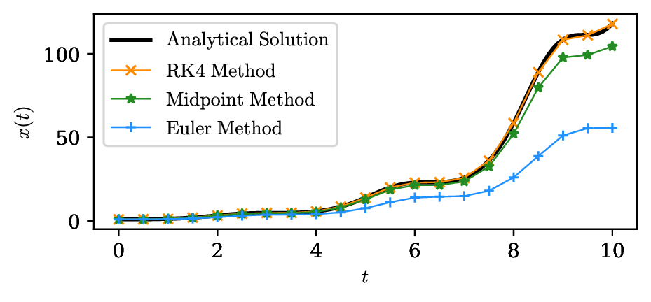
To compare the performance of these methods, we can visualize their outputs against the analytical solution:

It is important to highlight that advanced simulation techniques extend far beyond these numerical integration methods, allowing for the high-fidelity simulation of robotic systems, including visualization in pixel space. These techniques can incorporate detailed physical modeling, sensor data fusion, and learning-based approaches to create realistic and accurate simulations^†^†margin: One notable example is the use of Neural Radiance Fields (NeRFs) for generating photorealistic scenes. . As we will discuss in later chapters on perception, these advancements are crucial for tasks such as robot training, planning under uncertainty, and evaluating the autonomy stack in novel and previously unseen scenarios.

1.5 Summary

In this chapter, we introduced the fundamental principles underlying the modeling and simulation of robotic systems. We began by introducing state space models, which provide a mathematical framework to describe the evolution of a robot’s state over time. Next, we discussed a robot’s kinematics and dynamics, which characterize its motion and the constraints acting on it. This included a discussion of generalized coordinates and kinematic constraints—both holonomic and nonholonomic—along with the formulation of kinematic models using Pfaffian constraints. Throughout this chapter, we examined practical examples such as the rolling wheel, the pendulum, and wheeled robots like the unicycle and differential drive models. Finally, we introduced numerical integration techniques for simulating robot dynamics over time. We presented the Euler, Midpoint, and Runge-Kutta methods, highlighting their trade-offs and applications through concrete code examples.

To learn more.

For readers interested in a deeper and more rigorous treatment of the concepts presented in this chapter, Siciliano and Khatib (2007); Siciliano et al. (2008)³3. Siciliano, B., Khatib, O. Springer Handbook of Robotics. Springer-Verlag, 2007.
Siciliano, B., Sciavicco, L., Villani, L., Oriolo, G. Robotics: Modelling, Planning and Control. Springer Publishing Company, Incorporated, 2008. offer comprehensive and widely adopted references. These texts cover the mathematical foundations of robot kinematics, dynamics, and control in greater depth, and provide additional examples, derivations, and exercises that complement and extend the material introduced here.

1.6 Exercises

The starter code for the exercises provided below is available online through GitHub. To get started, download the code by running in a terminal window:

⬇

git clone https://github.com/StanfordASL/pora-exercises.git

We denote Problems requiring hand-written solutions and coding in Python with and , respectively.

Problem 1: Numerical Integration Methods

In the referenced algorithm we introduced a simple IVP and in Figure 1.7 we showed the differences between the Euler, midpoint, and fourth-order Runge-Kutta methods for solving it. In this exercise we will explore the use of a more advanced numerical integration scheme provided by the SciPy Python library called odeint. Open the notebook ch01/exercises/simulation.ipynb and practice by implementing the dynamics models for a damped pendulum and a bicycle, and then simulating them using odeint.

Problem 2: Nonholonomic Wheeled Robot Dynamics

The goal of this exercise is to familiarize yourself with some Python fundamentals that will be used throughout the book, such as NumPy and inheritance, as well as techniques for controlling nonholonomic wheeled robots.

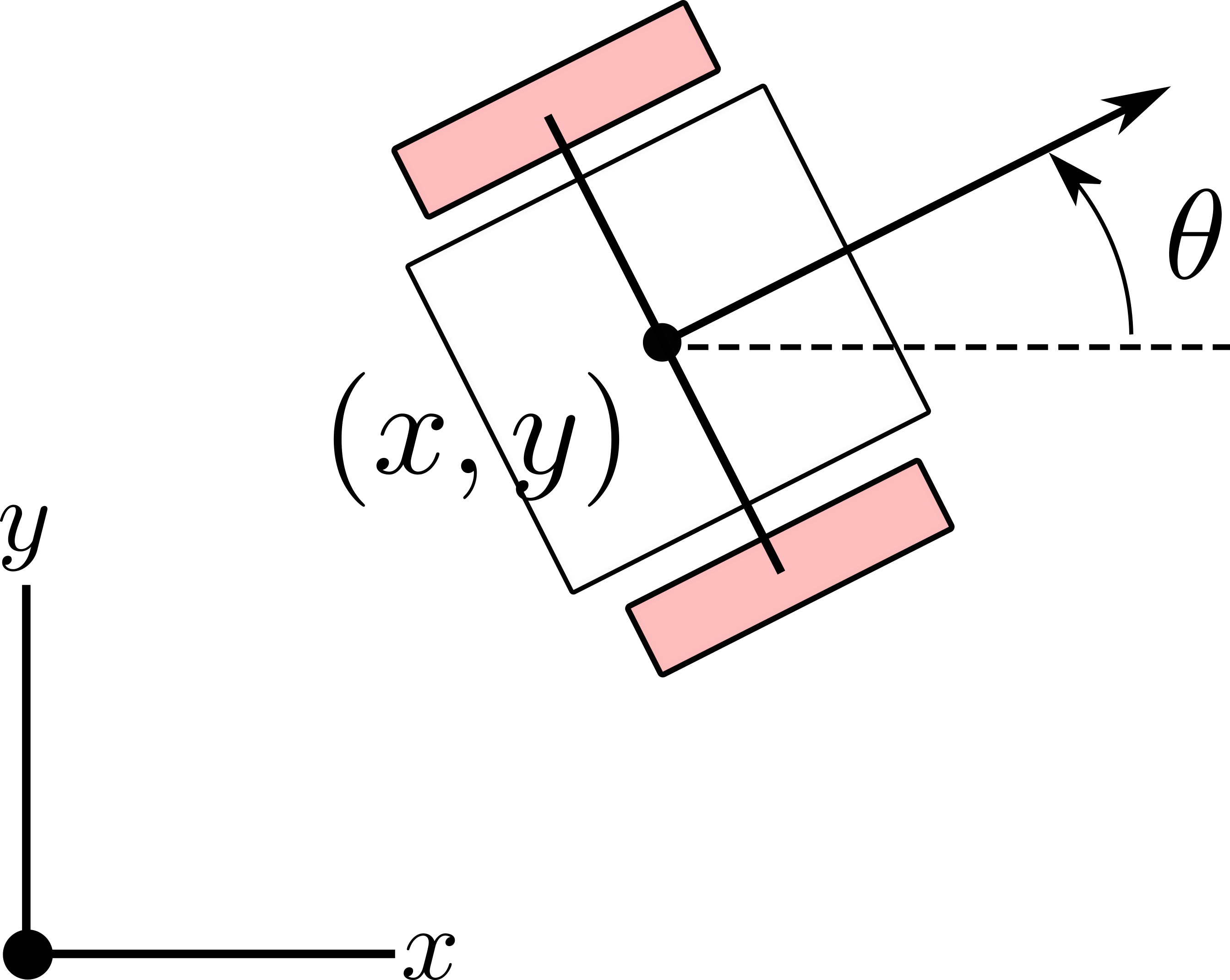
Consider a simple robot with two wheels whose state is defined by the position of the center of the axle and the heading angle, shown in Figure 1.8. This robot’s motion can be described by the simplest nonholonomic wheeled robot model, the unicycle model.

The kinematic model we will use reflects the rolling without side-slip constraint, and is given below in Equation 1.34.

\begin{split}\dot{x}(t)&=v(t)\cos(\theta(t)),\\ \dot{y}(t)&=v(t)\sin(\theta(t)),\\ \dot{\theta}(t)&=\omega(t).\end{split}

(1.34)

In this model, the robot state is $\bm{x}=[x,y,\theta]^{\top}$ , where $[x,y]^{\top}$ is the Cartesian location of the robot center and $\theta$ is its heading with respect to the $x$ -axis. The robot control inputs are $\bm{u}=[v,\omega]^{\top}$ , where $v$ is the velocity along the main axis of the robot and $\omega$ is the angular velocity, subject to the control constraints:

|v(t)|\leq 0.75\,\,\mathrm{m/s},\qquad\text{and}\qquad|\omega(t)|\leq 1.0\,\,% \mathrm{rad/s}.

In this problem, we will demonstrate the use of class inheritance in Python classes and the use of NumPy for vectorized operations. The notebook associated with this problem is ch01/exercises/nonholonomic_wheeled_robot_dynamics.ipynb.

We will be using a Dynamics base class for two different dynamics models: the wheeled robot dynamics model in this exercise and a double integrator model in the next exercise. The base class contains two unimplemented functions: step and rollout. The step function will propagate the dynamics a single time step with disturbances, and the rollout function will apply the step function multiple times to retrieve a trajectory of states over multiple time steps. Because the feed-forward dynamics are subject to disturbances, the same control sequence will result in different trajectories. We will observe this by executing multiple rollouts of the dynamics using the same control sequence from the same initial state.

In the ch01/exercises/nonholonomic_wheeled_robot_dynamics.ipynb notebook, complete the RobotDynamics class. Implement the function step using discrete-time Euler integration with the kinematic equations described in Equation 1.34. Then in the same class, implement the function rollout with two for-loops, calling the step function. Run the cells that rollout the robot’s dynamics and plot the control and state trajectories (this code has been written for you).

Problem 3: Double Integrator Dynamics

In this exercise, we consider the double integrator dynamics model:

\begin{split}\dot{x}(t)&=v_{x}(t),\\ \dot{y}(t)&=v_{y}(t),\\ \dot{v}_{x}(t)&=a_{x}(t),\\ \dot{v}_{y}(t)&=a_{y}(t).\end{split}

(1.35)

In this model, the robot state is $\bm{x}=[x,y,v_{x},v_{y}]^{\top}$ and the robot control inputs are $\bm{u}=[a_{x},a_{y}]^{\top}$ .

Notice that in the previous problem, we used a for-loop to rollout several trajectories of the robot’s dynamics. In this problem, we will use the same base dynamics class for a DoubleIntegratorDynamics class, and use batching to reduce the number of for-loops needed to perform multiple rollouts. The notebook for this problem is ch01/exercises/double_integrator_dynamics.ipynb.

i.

To reduce the number of for-loops needed to perform multiple rollouts, we will batch the dynamics equations applied in the function step. Implement the function step in the DoubleIntegratorDynamics class.
ii.

Fill in the code in function rollout in the DoubleIntegratorDynamics class using the step function you just wrote. Note that you should only need one for-loop!

Practice · 4 notebooks

Double Integrator Dynamics Open in Colab Source
Nonholonomic Wheeled Robot Dynamics Open in Colab Source
Simulation Open in Colab Source
Numerical Integration Open in Colab Source