Simultaneous Localization and Mapping (SLAM)

In Chapter 13, we studied robot localization under the assumption that a map of the environment, $\bm{m}$ , was known. While this assumption simplifies the estimation process, it is rarely met in practice. Robots often operate in a priori unknown or partially known environments. Examples include autonomous search-and-rescue in collapsed buildings, planetary exploration, and mapping of underwater structures. In such cases, a robot must concurrently infer its own state and build a map from noisy sensor data. This joint estimation problem is known as simultaneous localization and mapping (SLAM). The term SLAM and many classical algorithms were popularized by Thrun et al. (2005)¹1. Thrun, S., Burgard, W., Fox, D. Probabilistic Robotics. MIT Press, 2005., which remains a standard reference.

SLAM plays a central role in the perception and navigation layers of an autonomy stack. By providing a consistent, evolving spatial frame of reference, it allows downstream planning, control, and decision-making components to operate effectively in previously unseen environments.

The SLAM problem emerged in the late 1980s, with seminal contributions by Hugh Durrant-Whyte, John Leonard, and others, who framed it as a probabilistic joint estimation of pose and map. Early approaches treated SLAM as a large filtering problem. The EKF¹²12. Smith, Randall, Self, Matthew, Cheeseman, Peter. “Estimating uncertain spatial relationships in robotics.” In Autonomous robot vehicles, 167–193. Springer, 1990.
Leonard, John J, Durrant-Whyte, Hugh F. “Simultaneous map building and localization for an autonomous mobile robot..” In IROS, 1442–1447, 1991. provided a conceptually elegant way to maintain a joint Gaussian distribution over all robot poses and landmarks. In this formulation, the state vector contains the robot pose together with the positions of all $N$ landmarks, and the EKF maintains a $(3+2N)\times(3+2N)$ covariance matrix that encodes correlations between every pair of variables. As the map grows, storing and updating this dense covariance incurs $\mathcal{O}(N^{2})$ memory and computation, which quickly becomes prohibitive for large-scale mapping. Moreover, repeated linearization of nonlinear motion and measurement models around a single mean can introduce inconsistency and overly optimistic uncertainty estimates.

In the early 2000s, particle-filter methods, most notably FastSLAM¹³13. Montemerlo, Michael, Thrun, Sebastian, Koller, Daphne, Wegbreit, Ben et al. “FastSLAM: A factored solution to the simultaneous localization and mapping problem.” Aaai/iaai 593598(2), 593–598, 2002. offered a different perspective. By combining a particle-based representation of the robot’s trajectory with separate Gaussian estimates for individual landmarks (a technique known as Rao–Blackwellization), FastSLAM improved scalability and handled data association more flexibly. Here, data association refers to the problem of determining which previously mapped landmark, if any, corresponds to each new sensor measurement, an ambiguity that arises when multiple landmarks look similar or when sensing is noisy. At the same time, particle-filter approaches are susceptible to particle depletion. Over long trajectories, repeated weighting and resampling cause most particles to carry negligible weight, so that only a few distinct hypotheses effectively remain. When this happens, the particle set no longer provides a good approximation of the posterior, and the algorithm may become brittle unless many particles are used or more sophisticated proposal distributions are designed.

Subsequent work in the mid-2000s adopted an optimization-based view. Rather than updating a filter one step at a time, researchers formulated SLAM as a sparse nonlinear least-squares problem over a pose graph. In this representation, nodes correspond to robot poses and edges represent relative pose constraints obtained from odometry, loop closures, or scan matching. This graph-based SLAM perspective made it possible to exploit sparsity in the underlying problem, leverage robust cost functions to manage outliers, and apply incremental solvers for real-time operation^†^†margin: Representative systems include early pose-graph formulations by Lu and Milios (1997)²2. Lu, Feng, Milios, Evangelos. “Robot pose estimation in unknown environments by matching 2d range scans.” Journal of Intelligent and Robotic systems 18(3), 249–275, 1997., as well as modern optimization and incremental smoothing approaches such as square-root SAM ¹⁴14. Dellaert, Frank, Kaess, Michael. “Square root SAM: Simultaneous localization and mapping via square root information smoothing.” The International Journal of Robotics Research 25(12), 1181–1203, 2006., iSAM ¹⁵15. Kaess, Michael, Ranganathan, Ananth, Dellaert, Frank. “iSAM: Incremental smoothing and mapping.” IEEE Transactions on Robotics 24(6), 1365–1378, 2008., and g2o ¹⁶16. Kümmerle, Rainer, Grisetti, Giorgio, Strasdat, Hauke, Konolige, Kurt, Burgard, Wolfram. “g 2 o: A general framework for graph optimization.” In 2011 IEEE international conference on robotics and automation, 3607–3613, 2011.. . The factor-graph formalism further generalizes this idea: both robot poses and map variables are represented as nodes, while each measurement or prior contributes a factor, that is, a local term in the joint probability density that depends only on a small subset of variables. Factor graphs provide a unified way to encode heterogeneous constraints (from odometry to landmark observations and calibration parameters) in a single probabilistic model and now underpin most modern SLAM back-ends¹⁷17. Dellaert, Frank. “Factor graphs and GTSAM: A hands-on introduction.” Georgia Institute of Technology, Tech. Rep 2(4), 2012.
Dellaert, Frank. “Factor graphs: Exploiting structure in robotics.” Annual Review of Control, Robotics, and Autonomous Systems 4(1), 141–166, 2021..

Recent years have seen SLAM move beyond purely geometric mapping. Visual and visual–inertial SLAM, dense 3D reconstruction, semantic mapping, neural implicit representations (e.g., NeRF and Gaussian splatting), and learning-based front-ends all build on the same probabilistic foundations while extending the range of environments and tasks for which SLAM is viable. Modern SLAM systems combine probabilistic estimation, large-scale optimization, and learned representations, and are increasingly viewed as core components of broader “spatial AI” systems.

In the remainder of this chapter, we develop a unified view of SLAM that connects these ideas. Section 14.1 introduces the main algorithmic paradigms for SLAM, distinguishing filter-based and smoothing-based back-ends and clarifying the role each plays in modern systems. Next, we turn to the SLAM front-end in Section 14.2, describing how raw sensor data are converted into constraints, and then to modality-specific pipelines in Section 14.3, where we illustrate representative designs for visual, lidar, and radar SLAM. Building on this intuition, Section 14.4 formalizes SLAM as a Bayesian state estimation problem, introduces the underlying state-space models for motion and measurement, and derives the online and full SLAM formulations. The following sections instantiate this framework in concrete algorithms: EKF-SLAM in Section 14.5, particle-filter-based methods such as FastSLAM in Section 14.6, and optimization-based approaches including pose-graph SLAM and factor-graph SLAM in the referenced section. Finally, in Section 14.9 we survey advanced and emerging methods, dense and semantic mapping, neural implicit representations, and learning-based front-ends, and connect them to the broader vision of spatial AI.

14.1 SLAM Paradigms

Modern SLAM systems are typically organized into two conceptual layers. The front-end processes raw sensor data and extracts a set of constraints between states and map elements: features, correspondences, relative poses, and loop closures. Loop closures occur when the robot revisits a previously seen place and obtains a measurement that links two non-consecutive poses^†^†margin: For example, recognizing a corridor or room visited much earlier. , and these constraints are crucial for correcting accumulated drift. The back-end takes all these constraints and solves the underlying estimation problem, either recursively (filtering) or by optimizing over a window or the full trajectory (smoothing).

In this section, we focus on the back-end and distinguish two main paradigms: filter-based approaches and smoothing-based approaches. Both are grounded in the same probabilistic models introduced later in Section 14.4, but they make different choices about which variables to estimate explicitly and how to use past measurements.

14.1.1 Filter-based Approaches

Filter-based SLAM maintains a compact state estimate that is updated online as new sensor measurements arrive. The key idea is to propagate a belief over the current robot state and map using a recursive Bayes filter, without explicitly revisiting all past data at each step.

In EKF-SLAM, the robot state and map are stacked into a single augmented state vector, and the joint belief is modeled as a multivariate Gaussian. Motion and measurement models are linearized around the current estimate, and the EKF prediction–correction equations are applied at every time step (see the referenced section for the underlying EKF machinery). This yields an online algorithm that fuses information incrementally, but the covariance matrix is dense and of size $(n+2N)\times(n+2N)$ for $N$ landmarks and $n$ robot state variables. Storing and updating this matrix incurs $\mathcal{O}(N^{2})$ memory and computational cost, which becomes prohibitive as the map grows. Moreover, because non-linear motion and measurement models are repeatedly linearized around a single mean, linearization errors can accumulate over time and lead to inconsistent uncertainty estimates (see, for example, Thrun et al. (2005)³3. Thrun, S., Burgard, W., Fox, D. Probabilistic Robotics. MIT Press, 2005.).

Rao–Blackwellized particle filters, such as FastSLAM¹⁸18. Montemerlo, Michael, Thrun, Sebastian, Koller, Daphne, Wegbreit, Ben et al. “FastSLAM: A factored solution to the simultaneous localization and mapping problem.” Aaai/iaai 593598(2), 593–598, 2002., adopt a hybrid strategy. A particle filter represents the distribution over robot trajectories, while each particle carries separate Gaussian estimates for the landmarks. Conditioned on a sampled trajectory, the landmark estimates become conditionally independent, so that the map can be updated by running a set of tractable Kalman filters, specifically one per landmark, instead of one huge joint filter. This factorization dramatically reduces the cost per update and makes it easier to handle ambiguous data association. At the same time, particle-filter-based methods introduce new practical challenges, such as designing good proposal distributions, avoiding particle depletion over long trajectories, and maintaining global consistency. A detailed treatment of FastSLAM and Rao–Blackwellized particle filters can be found in Thrun et al. ¹⁹19. Thrun, S., Burgard, W., Fox, D. Probabilistic Robotics. MIT Press, 2005..

Filter-based methods are appealing when computation and memory budgets are tight, and when online operation with bounded per-step cost is a primary requirement. However, when long-term consistency, large-scale mapping, and aggressive loop closing are critical, they may struggle to fully exploit all available measurements, especially those that create strong constraints between distant poses.

14.1.2 Smoothing-based Approaches

Smoothing-based SLAM treats the entire robot trajectory and map as variables in a global estimation problem. Rather than maintaining only the current posterior $p(\bm{y}_{t}\mid\bm{z}_{1:t},\bm{u}_{1:t})$ , smoothing methods aim to recover either (i) the full posterior $p(\bm{y}_{1:t}\mid\bm{z}_{1:t},\bm{u}_{1:t})$ or (ii) a maximum a posteriori (MAP) estimate of the entire trajectory and map.

A convenient way to express this is through a graph representation with nodes and edges/factors.

•

Nodes represent unknown variables, such as robot poses at different times and landmark positions.
•

Edges or factors represent measurements or priors that relate a small subset of these variables: odometry constraints between consecutive poses, loop-closure constraints between non-consecutive poses, landmark observations that couple a pose to a landmark, and prior terms that anchor the map.

In a pose graph, nodes are pose variables and edges are relative pose constraints (odometry and loop closures). In a more general factor graph, both poses and map variables are nodes, and each measurement contributes a factor^†^†margin: A local term in the joint probability density that depends only on the variables involved in that measurement. .

From a probabilistic standpoint, each factor corresponds to a likelihood or prior term, and the overall objective (for MAP estimation) is to find the trajectory and map that best satisfy all factors simultaneously. Under Gaussian assumptions, this leads to a sparse nonlinear least-squares problem. The sparsity arises because each measurement involves only a few variables^†^†margin: For example, a single relative pose constraint involves two poses, and a landmark observation involves one pose and one landmark. , so the corresponding Jacobian and Hessian matrices contain many zeros. Modern sparse solvers exploit this structure to solve very large SLAM problems efficiently. References for graph- and factor-graph-based SLAM include Dellaert and Kaess (2006)⁴4. Dellaert, Frank, Kaess, Michael. “Square root SAM: Simultaneous localization and mapping via square root information smoothing.” The International Journal of Robotics Research 25(12), 1181–1203, 2006., Kaess et al. (2008)⁵5. Kaess, Michael, Ranganathan, Ananth, Dellaert, Frank. “iSAM: Incremental smoothing and mapping.” IEEE Transactions on Robotics 24(6), 1365–1378, 2008., and Kümmerle et al. (2011)⁶6. Kümmerle, Rainer, Grisetti, Giorgio, Strasdat, Hauke, Konolige, Kurt, Burgard, Wolfram. “g 2 o: A general framework for graph optimization.” In 2011 IEEE international conference on robotics and automation, 3607–3613, 2011..

Smoothing has two main advantages over pure filtering:

1.

It can re-linearize constraints in light of new data. When new measurements arrive, such as from a loop closure, the entire trajectory and map can be re-optimized, improving consistency relative to filters that only update the current state.
2.

It naturally incorporates loop closures by explicitly adding constraints between non-consecutive poses and adjusting the entire trajectory to satisfy them. This allows accumulated drift to be redistributed along the path when the robot revisits known areas.

14.1.3 Choosing a Paradigm

In practice, the choice between filtering and smoothing depends on several factors:

•

Real-time constraints. If strict real-time updates with tightly bounded per-step latency are required and computational resources are limited, filter-based approaches (EKF-SLAM, FastSLAM) are attractive.
•

Problem scale and loop closures. For large environments with many loop closures and long missions, smoothing- based methods and pose- or factor-graph formulations tend to yield more accurate and consistent maps, since they can re-optimize the full trajectory when new constraints arrive.
•

Implementation complexity. Filters are conceptually straightforward and often easier to implement for small systems. Graph-based methods require additional mathematical and software infrastructure^†^†margin: For example, sparse linear algebra and nonlinear optimization libraries. , but they are highly modular and extensible once in place.
•

Application priorities. Short-term navigation may prioritize fast local odometry and modest map maintenance, while long-term mapping, multi-session operation, and multi-robot scenarios benefit from the global consistency offered by smoothing and graph optimization.

In modern systems, the boundary between these paradigms is increasingly blurred. Incremental smoothing methods, such as iSAM²⁰20. Kaess, Michael, Ranganathan, Ananth, Dellaert, Frank. “iSAM: Incremental smoothing and mapping.” IEEE Transactions on Robotics 24(6), 1365–1378, 2008., provide real-time updates while retaining many of the advantages of batch optimization, and are widely used as SLAM back-ends in contemporary robotics libraries.

14.2 Front-End

So far, we have focused on back-end formulations: how to structure and solve the estimation problem once constraints are given. In a SLAM system, however, those constraints do not appear magically. They are distilled from raw sensor data by the front-end, which transforms pixels, point clouds, and other measurements into discrete relationships—such as relative poses, landmark observations, and loop closures—that the back-end subsequently enforces.

A useful way to think about this division of labor is the following. The back-end is the inference engine that reasons about the history of the robot’s motion and the structure of the environment, while the front-end is the perceptual pipeline that decides what information the back-end sees and how it is packaged. A strong back-end cannot compensate for a front-end that produces systematic outliers or weak, uninformative constraints.

At a high level, most SLAM front-ends can be understood as variants of the same conceptual pipeline:

1.

Feature extraction. Identify salient structures in the sensor data, such as keypoints, edges, geometric primitives, and learned descriptors.
2.

Data association. Decide which current features correspond to which previously seen features or map elements.
3.

Outlier rejection. Detect and remove inconsistent or spurious associations before they contaminate the estimate.
4.

Loop closure detection. Recognize previously visited places in order to add long-range constraints that correct drift.
5.

Scan alignment and registration. For range data, estimate relative poses between overlapping point clouds.

The detailed implementation of each stage depends strongly on the sensing modality^†^†margin: For example, cameras, lidar, radar, or others. , but their role in the SLAM system is shared: they determine which parts of the environment become landmarks or edges in the graph, how confidently we relate different poses, and when we introduce powerful loop-closure constraints. In the rest of this subsection, we briefly revisit these stages, connecting them to the perception tools developed in earlier chapters and emphasizing their global impact on SLAM.

14.2.1 Feature Extraction

From the SLAM perspective, feature extraction is the step where we decide which aspects of the environment will serve as “handles” for localization and mapping. This builds directly on the classical perception techniques of Chapter 8, which developed image filtering, edge and corner detection, descriptors, and geometric feature extraction, as well as the point cloud registration tools of the referenced section.^†^†margin: Deep learning architectures for perception, introduced in Chapter 9, provide learned alternatives to hand-designed features and are increasingly used in modern SLAM front-ends.

In visual SLAM, the front-end typically detects and describes repeatable image features—for example corners, blobs, or local patches—using classical methods such as Harris corners and SIFT-like descriptors, or modern learned features. These features are chosen to be robust to viewpoint and illumination changes so that they can be matched reliably across time and across cameras. The resulting 2D keypoints and descriptors form the basis for constructing geometric constraints—such as epipolar relations and reprojection errors—between camera poses and 3D landmarks, as discussed in Chapter 6 and Chapter 7.

In lidar-based SLAM, the analogous role is played by geometric primitives in point clouds: planes, edges, corner-like structures, or local surface patches. Extracting these primitives^†^†margin: For instance, using segmentation and model fitting methods from Chapter 8. provides stable anchor points that can be tracked across scans and used for scan-to-scan or scan-to-map registration.

For radar and other modalities, feature extraction must cope with lower resolution, clutter, and multipath. A common representation for automotive radars is the range–Doppler image: a 2D array obtained by applying Fourier transforms to the raw radar chirps, whose horizontal axis indexes range bins (distance from the sensor) and whose vertical axis indexes Doppler bins (radial velocity). Each pixel intensity reflects the strength of the return from targets at a given distance and relative speed, so a range–Doppler image can be viewed as a grayscale image that encodes both where objects are and how fast they are moving. In this representation, hand-crafted geometric cues are often combined with learned representations^†^†margin: For example, CNNs operating directly on range–Doppler images. to produce robust, repeatable signatures that can be matched over time.

14.2.2 Data Association

Once features have been extracted, the next crucial step is data association: determining whether a feature observed at time $t$ corresponds to a previously observed feature or map element. This is the mechanism by which we translate “this corner in the current image” into “the same corner we saw two seconds ago” or “landmark $m_{j}$ in the map”.

As in the localization setting in Chapter 13, data association is challenging: perceptual aliasing, sensor noise, occlusions, and environmental changes all make different places look similar, and the same place can look different over time. A correct association introduces a valid constraint between poses and landmarks, whereas an incorrect association can inject a large, systematically biased constraint that corrupts the entire estimate.

In practice, SLAM systems use a combination of techniques for data association, including:

•

Descriptor similarity, such as the distance in feature space for visual keypoints.
•

Geometric predictions from the current state estimate, such as projecting a landmark into the image or into a scan.
•

Probabilistic gating, where candidate matches are accepted only if they lie within an uncertainty-dependent region (often using Mahalanobis distance).
•

Higher-level cues, such as semantic labels like whether a feature belongs to a “door” object, or temporal consistency.

In many systems, data association is the most fragile component, but designing strategies with high recall (few missed true matches) and high precision (few false matches) is nonetheless critical for robust operation.

14.2.3 Outlier Rejection

Even with careful association, some matches will be wrong. The front-end must therefore include explicit mechanisms for identifying and rejecting outliers before they reach the back-end. This mirrors the geometric verification and model fitting pipelines discussed in Chapter 8^†^†margin: For example, RANSAC for line fitting or object pose estimation. , but now the models are camera geometry, relative poses, or scan alignment. Common strategies for outlier rejection include:

•

Geometric consistency checks, such as verifying that matched features satisfy epipolar constraints or that 3D-to-2D correspondences are compatible with a plausible camera pose.
•

Robust model fitting, for example using RANSAC and its variants to infer a relative pose or homography from putative matches while discarding outliers.
•

Statistical tests on residuals, where measurements whose errors are inconsistent with the expected covariance are discarded or downweighted.
•

Consistency with the current map, for instance requiring that new measurements be compatible with already-estimated landmarks and surfaces.

From the standpoint of the SLAM back-end, outlier rejection is not an optional cleanup step: a handful of large, unmodeled outliers can easily overwhelm even a sophisticated optimization or filtering algorithm.

14.2.4 Loop Closure Detection

A defining capability of SLAM systems is loop closure detection. Loop closure detection involves recognizing that the robot has returned to a previously visited place and generating a constraint that links the corresponding poses. From a global perspective, loop closures are the main tool for correcting accumulated drift: they tie together distant parts of the trajectory and allow the back-end to redistribute errors along the path.

Conceptually, loop closure detection extends data association from individual features to whole places. The front-end must answer questions like “does the current view correspond to some earlier pose $x_{k}$ ?” and, if so, “what is the relative transformation between $x_{t}$ and $x_{k}$ ?”. Typical loop closure pipelines involve the following steps:

1.

Constructing a compact descriptor for each place. For example, a bag-of-words representation over visual features, a global descriptor for a lidar scan, or a learned embedding from a neural network.
2.

Using this descriptor to retrieve a small set of candidate earlier poses that are likely to correspond to the same place.
3.

Verifying these candidates geometrically, such as by estimating a relative pose and checking the consistency of reprojection or registration errors.

Visual place-recognition methods (both classical and learned) and lidar scan descriptors (such as scan-context-style approaches) implement these ideas with different design choices and trade-offs between robustness, invariance, and computational cost.

Because each accepted loop closure introduces a long-range constraint in the graph, the stakes are high: a true loop closure can dramatically improve global consistency, whereas a false one can severely distort the map. For this reason, loop closure modules are often conservative, preferring to miss some potential closures rather than accept unreliable ones.

14.2.5 Scan Alignment and Iterative Closest Point (ICP)

In range-based SLAM, an additional central task is scan alignment: estimating the relative pose between overlapping point clouds or depth images. This aligns successive lidar sweeps, RGB-D frames, or accumulated submaps and provides relative pose constraints to the back-end.

the referenced section introduced the point cloud registration problem and the Iterative Closest Point (ICP) algorithm in detail. In the SLAM front-end, ICP and its many variants are used as a building block:

•

Given an initial guess for the relative pose between two scans (from odometry, IMU integration, or feature-based matching), ICP refines this guess by iteratively pairing points or primitives and solving for the rigid transformation that best aligns them.
•

The resulting transformation and its estimated uncertainty are then passed to the back-end as a relative pose constraint between the corresponding robot poses.

While conceptually simple and powerful, ICP is sensitive to initialization, can converge to local minima, and can be affected by outliers or partial overlap between scans. Modern SLAM systems therefore rarely rely on ICP alone: feature-based methods or learned global descriptors are used to obtain robust initial estimates and to reject poor matches, with ICP providing fine geometric refinement within a multi-stage registration pipeline.

14.2.6 Summary

Putting these pieces together, the front-end can be viewed as a modular pipeline that starts from raw sensor streams and outputs a set of carefully curated constraints: local feature-based measurements, loop-closure links, and scan-to-scan registrations, each with an associated uncertainty. In Section 14.3, we will see how this conceptual pipeline adapts to different sensing modalities, and in Section 14.4 we will formalize how these constraints enter the probabilistic SLAM model and drive the back-end algorithms developed in the remainder of the chapter.

14.3 SLAM Across Sensing Modalities

Up to this point, we have separated the SLAM problem into a front-end, which converts raw sensor observations into constraints, and a back-end, which estimates the trajectory and map given those constraints. In practice, the design of both components is strongly shaped by the available sensors. Cameras, lidar, and radar provide very different raw data, and thus require different feature extraction, data association, and loop-closure strategies, even though they ultimately feed the same types of constraints into the back-end.

In this section, we illustrate how the general front-end pipeline from Section 14.2 (feature extraction, data association, outlier rejection, loop closure, and scan alignment) specializes to three widely used sensing modalities: cameras (visual SLAM), lidar (lidar SLAM), and radar (radar SLAM). Our goal is not to cover each modality exhaustively, but to highlight how the same probabilistic ideas manifest in different front-end designs and what this implies for the back-end.

14.3.1 Vision-Based SLAM

Vision-based SLAM uses cameras as the primary source of information. Common configurations include monocular, stereo, and visual–inertial^†^†margin: Visual–inertial setups combine cameras with IMUs in a complementary way. setups. The raw input is a stream of images that the front-end must transform into geometric constraints between camera poses and 3D structure.

Front-end.

Building on the feature extraction and multi-view geometry tools from Chapter 6–Chapter 8, a typical visual front-end:

•

Detects and describes repeatable 2D features, such as corners, blobs, or local patches, using classical descriptors or learned features.
•

Matches features across frames to obtain 2D–2D or 2D–3D correspondences.
•

Estimates relative camera motion using geometric relations such as the essential matrix and the Perspective- $n$ -Point (PnP) model.
•

Performs outlier rejection, for example with RANSAC on the essential matrix or PnP residuals, and passes only geometrically consistent constraints to the back-end.
•

Runs place-recognition and geometric verification to propose and confirm loop closures.

Recall from Chapter 7 that, for calibrated cameras, the essential matrix $E=[t]_{\times}R$ encodes the epipolar constraint between two views: $p^{\top}Ep^{\prime}=0$ for corresponding normalized image points $p,p^{\prime}$ . Estimating $E$ from feature matches allows recovery of the relative rotation $R$ and translation direction $t$ between frames, up to scale. Similarly, the PnP problem (see Chapter 7) recovers the camera pose that best explains a set of 2D–3D correspondences between image points and map landmarks. In a SLAM front-end, these tools provide the relative pose edges and reprojection constraints that will later appear in the pose or factor graph.

For monocular cameras, the front-end must handle inherent scale ambiguity: relative motion can be recovered only up to an unknown scale until additional information resolves it^†^†margin: For example, from motion parallax, priors, or other sensors. . Stereo and visual–inertial setups reduce or remove this ambiguity by providing direct depth estimates or inertial motion constraints.

Back-end.

Visual SLAM back-ends commonly use sparse bundle adjustment or pose-graph optimization: frame-to-frame relative pose estimates, landmark reprojection errors, and inertial constraints are assembled into a single optimization problem. Systems such as PTAM²¹21. Klein, Georg, Murray, David. “Parallel tracking and mapping for small AR workspaces.” In 2007 6th IEEE and ACM international symposium on mixed and augmented reality, 225–234, 2007., ORB-SLAM²²22. Mur-Artal, Raul, Montiel, Jose Maria Martinez, Tardos, Juan D. “ORB-SLAM: A versatile and accurate monocular SLAM system.” IEEE transactions on robotics 31(5), 1147–1163, 2015., and VINS-Mono²³23. Qin, Tong, Li, Peiliang, Shen, Shaojie. “Vins-mono: A robust and versatile monocular visual-inertial state estimator.” IEEE transactions on robotics 34(4), 1004–1020, 2018. follow this design: a front-end that maintains a set of keyframes, tracks features, and proposes loop closures, coupled with a back-end that optimizes over camera poses (and possibly landmark positions) using the factor-graph machinery discussed in Section 14.1.

Perspective.

Vision-based SLAM excels at capturing rich appearance information and can be implemented with low-cost hardware, but it is sensitive to lighting changes, motion blur, and textureless scenes. These weaknesses motivate the use of robust front-end design and additional sensors such as IMUs and lidar.

14.3.2 Lidar-Based SLAM

Lidar sensors provide dense or semi-dense 3D point clouds that directly encode geometry. They are widely used in autonomous driving and field robotics, where accurate metric localization is required over large areas and in diverse conditions.

Front-end.

A typical lidar SLAM front-end includes:

•

Scan preprocessing, including deskewing and motion compensation, filtering, and ground removal.
•

Feature extraction, identifying edge-like or planar structures or small surface patches in the point cloud.
•

Scan alignment, using ICP or feature-based registration (building on the point cloud registration methods introduced in the referenced section).
•

Loop closure detection, often via global scan descriptors or learned embeddings that summarize the shape of a scan or local map.

ICP-based alignment provides relative pose constraints between consecutive scans (scan-to-scan) or between a scan and an accumulated submap (scan-to-map). Combining these with loop-closure constraints yields a rich set of geometric relationships between poses that the back-end can exploit.

Back-end.

On the back-end, pose-graph optimization is standard: nodes represent vehicle poses, and edges encode relative poses from scan registration and loop closures. Because lidar provides high-accuracy range data, even small misalignments can accumulate into significant drift if not corrected. Robust cost functions and outlier-resistant optimization strategies are therefore crucial. Incremental solvers allow these graphs to be updated in real time as new scans arrive.

Classic systems such as LOAM (lidar Odometry and Mapping)²⁴24. Zhang, Ji, Singh, Sanjiv et al. “LOAM: Lidar odometry and mapping in real-time..” In Robotics: Science and systems, 1–9, 2014. demonstrate how a carefully designed lidar front-end, coupled with a graph-based back-end, can achieve centimeter-level accuracy in real time.

Perspective.

Compared to cameras, lidar front-ends work with sparser but metrically precise data. They avoid some of the perceptual aliasing issues of vision, but introduce their own challenges in scan registration, handling dynamic objects, and coping with adverse weather or sensor artifacts.

14.3.3 Radar SLAM

Radar sensors, historically used in autonomy mainly for collision avoidance, are increasingly used for SLAM due to their robustness to fog, rain, dust, and poor lighting, and their long-range detection capabilities.

Front-end.

Radar returns are noisy, have lower angular resolution than cameras or lidar, and are degraded by multipath effects. As a result, feature extraction and data association are more challenging. Typical radar front-ends:

•

Compute range–Doppler or range–angle images from raw radar returns.
•

Extract prominent reflectors or local patterns as features, often using filtering and thresholding techniques adapted from Chapter 8.
•

Build global descriptors of scans or trajectories, or use learned embeddings tailored to radar data, to support place recognition and loop closure detection.
•

Estimate relative motions using registration in range–Doppler space, or by aligning reconstructed point clouds (when available), often in combination with inertial data.

Because of the high false-positive rate and spurious reflections, strong outlier rejection and conservative loop closure validation are especially important.

Back-end.

Back-end formulations for radar SLAM often mirror those of lidar SLAM: pose graphs whose edges come from radar-based relative pose estimates and loop closures. Recent systems frequently combine radar with other modalities, such as radar–inertial or radar–lidar odometry, to compensate for radar’s lower spatial resolution and to operate reliably in conditions where cameras and lidar are degraded.

Perspective.

Radar front-ends emphasize robustness over raw information density. When fused with other modalities, radar can significantly improve reliability in adverse conditions, which is increasingly important in safety-critical applications.

14.3.4 Discussion

Each sensing modality offers a different balance between richness of data, robustness, and environmental adaptability. Cameras provide dense appearance cues but can fail under challenging lighting or in texture-poor scenes. Lidar yields precise geometry but is more expensive and can be affected by adverse weather. Radar offers robustness and long range at the cost of sparser, noisier measurements and more difficult data association.

Modern SLAM systems therefore rarely rely on a single sensor. Instead, they combine complementary modalities—for example, visual–inertial odometry with lidar, or lidar with radar—so that the strengths of one sensor compensate for the weaknesses of another. This trend underscores the importance of the modular front-end and back-end architecture developed in the referenced section: front-ends can be adapted or extended as sensors change, while back-ends operate on a common abstraction of constraints.

In the next section, Section 14.4, we temporarily abstract away these modality-specific details and formalize SLAM as a Bayesian state estimation problem. There, we introduce the motion and measurement models that underlie both filtering and smoothing formulations, and show how the constraints produced by the various front-ends enter the probabilistic SLAM framework.

14.4 Mathematical Foundations of SLAM

Equipped with an understanding of the front-end, we can now formalize the SLAM problem as a Bayesian state estimation problem. This formal viewpoint captures, in a single probabilistic model, how the robot state evolves over time and how the map of the environment is refined as new data arrive. It also provides the bridge between the front-end constraints and the filtering- and smoothing-based back-ends discussed in Section 14.1.

Throughout this section we assume that the map $\bm{m}$ is static over the time horizon of interest: walls do not move, landmarks remain fixed, and the environment does not change in ways that must be explicitly modeled. This assumption is appropriate for many indoor and urban scenarios and keeps the notation manageable. Extensions to dynamic maps—for example, modeling moving objects or slowly changing geometry—typically augment the state with additional variables for dynamic entities and introduce explicit time-dependence in the map; we briefly return to these ideas in later chapters.

Formally, given a sequence of control inputs $\bm{u}_{1:t}$ and sensor measurements $\bm{z}_{1:t}$ , the SLAM problem asks the robot to estimate both its trajectory $\bm{x}_{1:t}$ (or at least its current state $\bm{x}_{t}$ ) and the map $\bm{m}$ of the environment. As in Chapter 13, we treat $\bm{x}_{t}\in\mathbb{R}^{n}$ as the robot state at time $t$ , typically including pose and possibly velocity or other motion-related variables. The map $\bm{m}$ encodes properties of the environment according to a chosen representation. We reuse the same families of map models introduced in Chapter 13, namely feature-based, dense/grid-based, and hybrid maps, which can include sparse sets of landmarks, occupancy grids or signed distance fields, and combinations thereof for systems that require both long-range localization and detailed local geometry.

Since the goal is to estimate both the robot state and the map, it is convenient to combine them into a single joint state at time $t$ :

\bm{y}_{t}\coloneqq\left(\bm{x}_{t},\bm{m}\right),

and we denote the joint state trajectory by:

\bm{y}_{1:t}\coloneqq\left(\bm{y}_{1},\ldots,\bm{y}_{t}\right).

Two closely related formulations are particularly important in practice.

Definition 14.1 (Online SLAM.).

The goal of online SLAM is to estimate the current robot state together with the map. Mathematically, this corresponds to the belief:

\text{bel}(\bm{y}_{t})=p(\bm{y}_{t}\mid\bm{z}_{1:t},\bm{u}_{1:t}).

(14.1)

Definition 14.2 (Full SLAM.).

The goal of full SLAM is to estimate the entire trajectory of the robot together with the map. Mathematically, this corresponds to the belief:

\text{bel}(\bm{y}_{1:t})=p(\bm{y}_{1:t}\mid\bm{z}_{1:t},\bm{u}_{1:t}).

(14.2)

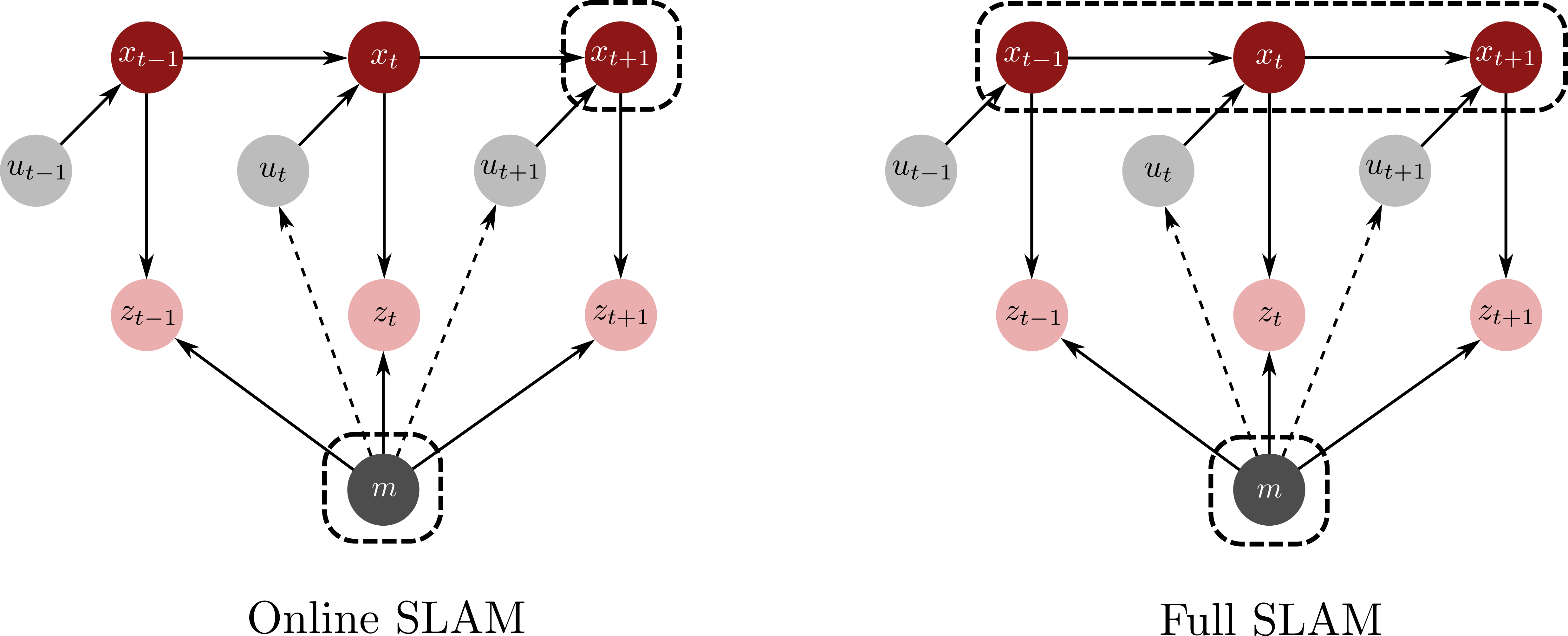
The distinction between these two viewpoints is illustrated in Figure 14.1. Online SLAM focuses on the most recent pose and the map, which is often what is needed for real-time control and navigation. Full SLAM retains the entire pose history, which is particularly useful for building globally consistent maps, enforcing loop closures, or performing offline analysis over long missions.

In both cases, localization and mapping are tightly coupled: accurate localization requires an accurate map, and accurate mapping depends on reliable localization. This interplay makes SLAM sensitive to drift, data association errors, and outliers—issues that modern algorithms address via loop closure detection, robust front-ends, and global optimization in the back-end.

Refer to caption — Figure 14.1: Online SLAM problems estimate only the current robot state together with the map, whereas full SLAM problems estimate the entire trajectory of past robot states (the state history) along with the map.

14.4.1 Motion and Measurement Models

To connect controls, states, and measurements in a probabilistic framework, we must first specify models for how the robot moves and how its sensors behave.

At each time step $t$ , the robot receives:

•

A control input $\bm{u}_{t}$ , such as wheel velocities, steering commands, thrust forces.
•

Sensor observations $\bm{z}_{t}$ , such as lidar scans, images, range–bearing measurements.

The full histories up to time $t$ are denoted by $\bm{u}_{1:t}=\left(\bm{u}_{1},\ldots,\bm{u}_{t}\right)$ and $\bm{z}_{1:t}=\left(\bm{z}_{1},\ldots,\bm{z}_{t}\right)$ .

The robot’s motion is captured by a state transition model:

\bm{x}_{t+1}=f(\bm{x}_{t},\bm{u}_{t})+\bm{\epsilon}_{t},

where $f(\cdot)$ encodes the deterministic dynamics and $\bm{\epsilon}_{t}$ is stochastic process noise with distribution $p(\bm{\epsilon}_{t})$ . The term $\bm{\epsilon}_{t}$ accounts for unmodeled effects such as slippage, disturbances, or modeling errors.

Sensor observations are modeled by a measurement function:

\bm{z}_{t}=h(\bm{x}_{t},\bm{m})+\bm{\delta}_{t},

where $h(\cdot)$ maps the robot state and map to an ideal, noise-free measurement, and $\bm{\delta}_{t}$ is measurement noise with distribution $p(\bm{\delta}_{t})$ . This noise captures sensor imperfections and environmental effects, such as reflections, lighting changes, and occlusions.

Both motion and measurement models may be linear or nonlinear, depending on the sensing and actuation setup. A few simple examples illustrate this variety:

Example 14.4.1 (Linear motion model (odometry).).

For a differential-drive robot with small wheel slippage, the dynamics can be approximated as:

\bm{x}_{t+1}=\bm{x}_{t}+B\bm{u}_{t}+\bm{\epsilon}_{t},

where $B$ is a constant matrix mapping wheel velocities $\bm{u}_{t}$ to pose increments.

Example 14.4.2 (Nonlinear motion model (unicycle).).

A more realistic planar model uses the robot’s heading:

	$\displaystyle x_{t+1}$	$\displaystyle=x_{t}+V_{t}\cos(\theta_{t})\Delta t+w_{t}^{x},$
	$\displaystyle y_{t+1}$	$\displaystyle=y_{t}+V_{t}\sin(\theta_{t})\Delta t+w_{t}^{y},$
	$\displaystyle\theta_{t+1}$	$\displaystyle=\theta_{t}+\omega_{t}\Delta t+w_{t}^{\theta},$

where $V_{t}$ and $\omega_{t}$ are commanded linear and angular velocities and $w_{t}^{x},w_{t}^{y},w_{t}^{\theta}$ represent process noise.

Example 14.4.3 (Linear measurement model (1D range).).

If a robot moves along a line and measures the distance to a fixed landmark at position $m$ , then:

z_{t}=m-x_{t}+v_{t},

which is linear in $x_{t}$ .

Example 14.4.4 (Nonlinear measurement model (range–bearing in 2D).).

For a landmark at position $\left(m_{x},m_{y}\right)$ , the sensor might return range and bearing:

	$\displaystyle r_{t}$	$\displaystyle=\sqrt{(m_{x}-x_{t})^{2}+(m_{y}-y_{t})^{2}}+\delta_{t}^{r},$
	$\displaystyle\phi_{t}$	$\displaystyle=\operatorname{atan2}(m_{y}-y_{t},m_{x}-x_{t})-\theta_{t}+\delta_% {t}^{\phi},$

which is nonlinear in the robot pose and landmark coordinates.

Example 14.4.5 (Nonlinear measurement model (camera projection).).

A 3D landmark $\left(X,Y,Z\right)$ projects to image coordinates via:

\begin{bmatrix}u\\ v\end{bmatrix}=\frac{1}{Z}\begin{bmatrix}f_{x}&0&c_{x}\\ 0&f_{y}&c_{y}\end{bmatrix}\begin{bmatrix}X\\ Y\\ Z\end{bmatrix}+\bm{\delta}_{t},

where $f_{x},f_{y}$ are focal lengths and $c_{x},c_{y}$ the principal point. The division by $Z$ makes the model nonlinear.

These models, together with the choice of map representation, fully specify the probabilistic SLAM problem.

14.4.2 Bayesian Formulation of SLAM

From a Bayesian perspective, SLAM is a problem of inferring unknown quantities (the trajectory and map) from known data (controls and measurements), given probabilistic models for motion and sensing.

Using Bayes’ rule, the full SLAM posterior can be written as:

p(\bm{y}_{1:t}\mid\bm{z}_{1:t},\bm{u}_{1:t})\propto p(\bm{z}_{1:t}\mid\bm{y}_{% 1:t},\bm{u}_{1:t})\;p(\bm{y}_{1:t}\mid\bm{u}_{1:t}),

(14.3)

where:

•

$p(\bm{z}_{1:t}\mid\bm{y}_{1:t},\bm{u}_{1:t})$ is the likelihood, which encodes how probable the sensor data are given a particular trajectory and map; and
•

$p(\bm{y}_{1:t}\mid\bm{u}_{1:t})$ is the prior, which captures knowledge about how the system evolves under the controls, as well as any prior assumptions on the map.

The distinction between online and full SLAM discussed above is reflected in where we place the focus: online SLAM is concerned with the marginal $p(\bm{y}_{t}\mid\bm{z}_{1:t},\bm{u}_{1:t})$ , obtained by integrating out past states from Equation 14.3, whereas full SLAM keeps the entire path $p(\bm{y}_{1:t}\mid\bm{z}_{1:t},\bm{u}_{1:t})$ . In the remainder of the chapter, we start from this Bayesian formulation and derive classical solutions: EKF-SLAM for online SLAM and FastSLAM for full SLAM. We then move on to modern graph-based approaches, robust optimization, and registration methods such as ICP and bundle adjustment, which can be interpreted as optimization-based approximations to the same underlying posterior.

14.4.3 State-space Factorization for SLAM

Direct computation of the SLAM posterior is intractable in all but the simplest cases. However, the problem becomes manageable once we exploit conditional independencies implied by the motion and measurement models.

The key assumption is the Markov property of the dynamics: the future depends on the past only through the present state. For the motion model, this gives:

p(\bm{x}_{t+1}\mid\bm{x}_{1:t},\bm{m},\bm{u}_{1:t})=p(\bm{x}_{t+1}\mid\bm{x}_{% t},\bm{u}_{t}),

which states that the next state depends only on the current state and the latest control. Similarly, for the measurement model we assume:

p(\bm{z}_{t}\mid\bm{x}_{1:t},\bm{m},\bm{z}_{1:t-1},\bm{u}_{1:t})=p(\bm{z}_{t}% \mid\bm{x}_{t},\bm{m}),

meaning that the current measurement depends only on the current state and the map, not on the full history.

Under these assumptions, the posterior for full SLAM factors as:

p(\bm{x}_{1:t},\bm{m}\mid\bm{z}_{1:t},\bm{u}_{1:t})\propto\eta\,p(\bm{x}_{1})p% (\bm{m})\prod_{i=1}^{t}p(\bm{z}_{i}\mid\bm{x}_{i},\bm{m})\prod_{i=1}^{t-1}p(% \bm{x}_{i+1}\mid\bm{x}_{i},\bm{u}_{i}),

(14.4)

where $p(\bm{x}_{1})$ is the prior over the initial state, $p(\bm{m})$ is the prior over the map, and $\eta$ is a normalization constant. Each factor in this expression corresponds directly to one of the components of the SLAM model:

•

$p(\bm{x}_{i+1}\mid\bm{x}_{i},\bm{u}_{i})$ is a motion factor (odometry, IMU, …).
•

$p(\bm{z}_{i}\mid\bm{x}_{i},\bm{m})$ is a measurement factor (range–bearing, image reprojection, scan alignment, …).
•

$p(\bm{x}_{1})$ and $p(\bm{m})$ are prior factors that anchor the solution.

This factorization is the state-space version of the graphical models discussed in Section 14.1. It underlies both filtering-based and smoothing-based methods:

•

Filtering. Filtering-based methods marginalize out older states to maintain a belief over the current state and map:

$\text{bel}(\bm{x}_{t},\bm{m})\;\coloneqq\;p(\bm{x}_{t},\bm{m}\mid\bm{z}_{1:t},% \bm{u}_{1:t}),$

and update it as new controls and measurements arrive. Applying Bayes’ rule and the Markov assumptions yields the familiar Bayes-filter recursion:

Prediction (motion update):

$\overline{\text{bel}}(\bm{x}_{t+1},\bm{m})=\int p(\bm{x}_{t+1}\mid\bm{x}_{t},% \bm{u}_{t})\;\text{bel}(\bm{x}_{t},\bm{m})\;d\bm{x}_{t},$

Correction (measurement update):

$\text{bel}(\bm{x}_{t+1},\bm{m})=\eta\,p(\bm{z}_{t+1}\mid\bm{x}_{t+1},\bm{m})\;% \overline{\text{bel}}(\bm{x}_{t+1},\bm{m}),$

where $\eta$ normalizes the belief to integrate to $1$ .
•

Smoothing. Smoothing-based methods operate directly on Equation 14.4, keeping the entire trajectory $\bm{x}_{1:t}$ and map $\bm{m}$ as variables. Under Gaussian assumptions, maximizing the posterior $p(\bm{x}_{1:t},\bm{m}\mid\bm{z}_{1:t},\bm{u}_{1:t})$ is equivalent to solving a sparse nonlinear least-squares problem whose terms correspond to the factors in Equation 14.4—this is the optimization viewpoint developed in the referenced section.

The rest of this chapter introduces what can be interpreted as different ways of approximating and exploiting this factorization:

•

EKF-SLAM (Section 14.5) implements the Bayes-filter recursion directly under Gaussian noise and first-order linearization.
•

FastSLAM and related particle-filter methods (Section 14.6) use sampling over trajectories combined with conditional Gaussian subproblems for map features.
•

Graph- and factor-graph-based SLAM (the referenced section) encode the factors in Equation 14.4 explicitly in a graphical model and solve for a MAP estimate via sparse nonlinear optimization.

In each case, the underlying probabilistic structure is the same; what differs is how we represent the belief and which approximations we make to render computation tractable.

14.5 Extended Kalman Filter SLAM

We have already encountered the EKF in two contexts: first as a general state estimation algorithm in Chapter 12, and then as a localization method when a map is known in Chapter 13. We now extend this idea to the SLAM setting.

In EKF-SLAM, the map is treated as part of an augmented state vector, and the joint posterior over robot pose and map is updated recursively under Gaussian noise assumptions and first-order linearizations of the process and measurement models²⁵25. Smith, Randall, Self, Matthew, Cheeseman, Peter. “Estimating uncertain spatial relationships in robotics.” In Autonomous robot vehicles, 167–193. Springer, 1990.
Leonard, John J, Durrant-Whyte, Hugh F. “Simultaneous map building and localization for an autonomous mobile robot..” In IROS, 1442–1447, 1991.. This generalizes the earlier uses of the EKF from estimating only the robot’s state to simultaneously estimating a static feature-based map and the evolving trajectory.

As in Chapter 13, we assume that the map is feature-based:

\bm{m}=\{m_{1},m_{2},\dots,m_{N}\},

where $m_{i}$ is the $i$ -th feature with coordinates $\left(m_{i,x},m_{i,y}\right)$ in a 2D environment. The joint state vector at time $t$ is then:

\bm{y}_{t}\coloneqq\begin{bmatrix}\bm{x}_{t}\\ \bm{m}\end{bmatrix},

(14.5)

and the online SLAM goal is to compute the posterior belief:

\text{bel}(\bm{y}_{t})=p(\bm{x}_{t},\bm{m}\mid\bm{z}_{1:t},\bm{u}_{1:t}).

We consider a state transition model for the augmented state $\bm{y}_{t}$ of the form:

\bm{y}_{t}=g(\bm{y}_{t-1},\bm{u}_{t})+\bm{\epsilon}_{t},

with additive Gaussian process noise $\bm{\epsilon}_{t}\sim\mathcal{N}(\bm{0},Q_{t})$ . The nonlinear function $g$ is defined as:

g(\bm{y}_{t-1},\bm{u}_{t})=\begin{bmatrix}f(\bm{x}_{t-1},\bm{u}_{t})\\ m_{1,t-1}\\ \vdots\\ m_{N,t-1}\end{bmatrix},

where $f$ denotes the robot motion model, and we assume that each map feature $m_{i}$ is static, so its process model is the identity. The process noise covariance has block structure:

Q_{t}=\begin{bmatrix}\tilde{Q}_{t}&0\\ 0&0\end{bmatrix},

where $\tilde{Q}_{t}$ is the motion model noise covariance for the robot, and the zero blocks reflect the assumption of no process noise for the map features.

The Jacobian of the augmented motion model is:

G_{t}=\nabla_{\bm{y}}g(\bm{y},\bm{u}_{t})\big{|}_{\bm{y}=\bm{\mu}_{t-1}},

that is, the derivative of $g$ with respect to the augmented state, evaluated at the current mean estimate $\bm{\mu}_{t-1}$ .

The measurement model mirrors the localization setting in Chapter 13:

\bm{z}^{i}_{t}=h(\bm{y}_{t},j)+\bm{\delta}_{t},

where $\bm{\delta}_{t}\sim\mathcal{N}(\bm{0},R_{t})$ is zero-mean Gaussian noise and $j$ is the index of the map feature $m_{j}\in\bm{m}$ associated with measurement $i$ . The Jacobian of the measurement model is:

H^{j}_{t}=\nabla_{\bm{y}}h(\bm{y},j)\big{|}_{\bm{y}=\bar{\bm{\mu}}_{t}},

the derivative of the measurement function with respect to the augmented state, evaluated at the predicted mean $\bar{\bm{\mu}}_{t}$ obtained from the EKF prediction step.

14.5.1 EKF-SLAM with Known Correspondences

As in EKF localization, it is instructive to first consider the case in which the data associations are known. Let $\bm{c}_{t}=[c_{t}^{1},\dots]^{\top}$ denote the correspondence vector, where $c_{t}^{i}$ is the index of the map feature associated with measurement $\bm{z}_{t}^{i}$ . With known correspondences, the EKF-SLAM algorithm shown in Algorithm 1 is nearly identical to the EKF localization algorithm in the referenced algorithm, except that it operates on the augmented state $\bm{y}$ containing both robot pose and map.

Data:

\bm{\mu}_{t-1},\Sigma_{t-1},\bm{u}_{t},\bm{z}_{t},\bm{c}_{t}

Result:

\bm{\mu}_{t},\Sigma_{t}

// Prediction step: propagate belief with motion model

\bar{\bm{\mu}}_{t}=g(\bm{\mu}_{t-1},\bm{u}_{t})

\bar{\Sigma}_{t}=G_{t}\Sigma_{t-1}G_{t}^{T}+Q_{t}

// Correction step: process each measurement

foreach $\bm{z}_{t}^{i}$ do

j=c_{t}^{i}

// index of associated map feature

if feature $j$ has never been seen before then

Initialize

\begin{bmatrix}\bar{\mu}_{j,x}\\\bar{\mu}_{j,y}\end{bmatrix}

as the expected position based on

\bm{z}_{t}^{i}

// Innovation covariance

S_{t}^{i}=H_{t}^{j}\bar{\Sigma}_{t}[H^{j}_{t}]^{T}+R_{t}

// Kalman gain

K^{i}_{t}=\bar{\Sigma}_{t}[H^{j}_{t}]^{T}[S_{t}^{i}]^{-1}

// State update using measurement residual

\bar{\bm{\mu}}_{t}=\bar{\bm{\mu}}_{t}+K^{i}_{t}(\bm{z}^{i}_{t}-h(\bar{\bm{\mu}%}_{t},j))

// Covariance update

\bar{\Sigma}_{t}=(I-K^{i}_{t}H^{j}_{t})\bar{\Sigma}_{t}

// Final posterior belief

\bm{\mu}_{t}=\bar{\bm{\mu}}_{t}

\Sigma_{t}=\bar{\Sigma}_{t}

return

\bm{\mu}_{t},\Sigma_{t}

Algorithm 1 EKF Online SLAM with Known Correspondences

A typical initialization for the belief $\text{bel}(\bm{y}_{0})$ places the robot at the origin of the map frame with high confidence and assigns very weak priors to the features:

\bm{\mu}_{0}=\begin{bmatrix}\bm{x}_{0}\\ 0\\ \vdots\\ 0\end{bmatrix},\quad\Sigma_{0}=\begin{bmatrix}\tilde{\Sigma}_{0}&0&\cdots&0\\ 0&\infty&\cdots&0\\ \vdots&\vdots&\ddots&\vdots\\ 0&0&\cdots&\infty\\ \end{bmatrix},

where:

\bm{x}_{0}=\begin{bmatrix}0\\ \vdots\\ 0\end{bmatrix},\quad\tilde{\Sigma}_{0}=\begin{bmatrix}0&\cdots&0\\ \vdots&\ddots&\vdots\\ 0&\cdots&0\end{bmatrix},

and $\bm{x}_{0}$ and $\tilde{\Sigma}_{0}$ are the initial robot state and its covariance. The large feature covariance terms—conceptually infinite—express complete lack of prior knowledge about landmark locations. When a feature is first observed, the algorithm reinitializes its mean using the corresponding measurement, rather than linearizing the measurement function about an arbitrary initial guess such as the origin.

For a range–bearing sensor in 2D, the geometry is simple. Suppose the robot pose is $(x_{t},y_{t},\theta_{t})$ in the global frame, and the sensor returns a range $r$ and bearing $\varphi$ to a previously unseen feature in the robot frame. In the robot frame, the feature lies at:

\begin{bmatrix}r\cos\varphi\\ r\sin\varphi\end{bmatrix}.

To express this in the global frame, we first rotate by the robot heading $\theta_{t}$ and then translate by the robot position:

\begin{bmatrix}m_{x}\\[1.99997pt] m_{y}\end{bmatrix}=\begin{bmatrix}x_{t}\\[1.99997pt] y_{t}\end{bmatrix}+\begin{bmatrix}\cos\theta_{t}&-\sin\theta_{t}\\ \sin\theta_{t}&\cos\theta_{t}\end{bmatrix}\begin{bmatrix}r\cos\varphi\\[1.9999% 7pt] r\sin\varphi\end{bmatrix}.

Using trigonometric identities, this simplifies to:

m_{x}=x_{t}+r\cos(\theta_{t}+\varphi),\qquad m_{y}=y_{t}+r\sin(\theta_{t}+% \varphi).

This is the formula used in the algorithm to initialize a landmark from a single range–bearing observation. Because the sensor provides both range and bearing, a single measurement suffices to place the landmark (up to measurement noise). By contrast, for pure-bearing sensors such as a monocular camera without depth information, multiple views and robot motion are required to infer landmark positions, as discussed in the visual SLAM examples of Section 14.3.

14.5.2 EKF-SLAM with Unknown Correspondences

So far, we have assumed that each measurement $\bm{z}_{t}^{i}$ is already matched to a map feature via a correspondence index $c_{t}^{i}$ . In reality, these correspondences are rarely known and must be inferred online. This makes SLAM substantially harder than the known-map localization problem in Chapter 11 because the map itself is uncertain.

Conceptually, the main new task is to decide, for every incoming measurement, whether it should be assigned to an existing feature (data association) or interpreted as a new feature (map expansion). Both choices affect subsequent estimates: an incorrect association can corrupt the map, while an unnecessary new feature increases complexity.

A common strategy is to choose correspondences by maximum likelihood. For each measurement $\bm{z}_{t}^{i}$ , we evaluate its likelihood under each possible landmark hypothesis and select the most plausible one.

Given a predicted belief $\overline{\text{bel}}(\bm{y}_{t})$ after the motion update, the predictive distribution for a measurement $\bm{z}_{t}^{i}$ associated with landmark $j$ is the distribution of $\bm{z}_{t}^{i}$ implied by the current uncertainty over $\bm{y}_{t}$ and the measurement model. Formally:

p(\bm{z}_{t}^{i}\mid\bm{z}_{1:t-1},\bm{u}_{1:t},c_{t}^{i}=j)=\int p(\bm{z}_{t}% ^{i}\mid\bm{y}_{t},c_{t}^{i}=j)\;\overline{\text{bel}}(\bm{y}_{t})\,d\bm{y}_{t}.

Under the EKF assumptions of a Gaussian belief and linearized measurement model, this integral can be computed in closed form and yields a likelihood Gaussian distribution $\mathcal{N}(\bm{z}_{t}^{i}\mid\hat{\bm{z}}_{t}^{j},S_{t}^{j})$ with mean:

\hat{\bm{z}}_{t}^{j}=h(\bar{\bm{\mu}}_{t},m_{j}),

and covariance:

S_{t}^{j}=H_{t}^{j}\bar{\Sigma}_{t}[H_{t}^{j}]^{\top}+R_{t},

exactly as in the EKF localization case.

Maximizing this likelihood with respect to $j$ is equivalent (see Chapter 11) to minimizing the Mahalanobis distance:

d_{t}^{ij}=(\bm{z}_{t}^{i}-\hat{\bm{z}}_{t}^{j})^{\top}[S_{t}^{j}]^{-1}(\bm{z}% _{t}^{i}-\hat{\bm{z}}_{t}^{j}).

(14.6)

Intuitively, $d_{t}^{ij}$ measures how many “standard deviations” the actual measurement $\bm{z}_{t}^{i}$ lies from the predicted measurement $\hat{\bm{z}}_{t}^{j}$ , taking into account the full covariance. Compared to Euclidean distance, the Mahalanobis distance automatically downweights directions of high uncertainty and emphasizes directions of low uncertainty.

Decision rule and $\chi^{2}$ gating.

The unknown-correspondence EKF-SLAM loop adds one more decision layer on top of Algorithm 1:

1.

For each measurement $\bm{z}_{t}^{i}$ , hypothesize a potential new feature position, for example by triangulating from range–bearing measurements, which would increase the feature count from $N_{t-1}$ to $N_{t}=N_{t-1}+1$ .
2.

For all existing features $k=1,\ldots,N_{t}$ , compute the Mahalanobis distance $d_{t}^{ik}$ between $\bm{z}_{t}^{i}$ and the prediction for feature $k$ :

$\hat{\bm{z}}_{t}^{k}=h(\bar{\bm{\mu}}_{t},k),\qquad S_{t}^{k}=H_{t}^{k}\bar{% \Sigma}_{t}[H_{t}^{k}]^{T}+R_{t},$

and:

$d_{t}^{ik}=(\bm{z}_{t}^{i}-\hat{\bm{z}}_{t}^{k})^{\top}[S_{t}^{k}]^{-1}(\bm{z}% _{t}^{i}-\hat{\bm{z}}_{t}^{k}).$
3.

If all $d_{t}^{ik}$ are “too large”, treat $\bm{z}_{t}^{i}$ as a new feature; otherwise, assign the measurement to the feature with the smallest Mahalanobis distance.

To formalize the notion of “too large”, it is common to use a $\chi^{2}$ gate. For a $d$ -dimensional measurement and a correctly specified Gaussian model, the Mahalanobis distance $d_{t}^{ij}$ follows a $\chi^{2}$ distribution with $d$ degrees of freedom. This means that if a landmark hypothesis is correct, $d_{t}^{ij}$ will lie below a chosen threshold most of the time. We therefore pick a threshold $\alpha$ such that:

\Pr\bigl{[}\chi^{2}_{d}\leq\alpha\bigr{]}=p,

where $p$ is a desired confidence level, such as $p=0.95$ . The region $d_{t}^{ij}\leq\alpha$ is then a $p$ -confidence “ellipse” in measurement space: we accept an association only if the measurement falls inside this ellipse. In practice:

•

If $d_{t}^{ik}\leq\alpha$ for some $k$ , we select the feature with the smallest $d_{t}^{ik}$ as the best match.
•

If $d_{t}^{ik}>\alpha$ for all existing features, we consider $\bm{z}_{t}^{i}$ to be a new landmark and initialize it accordingly.

The complete EKF-SLAM algorithm for unknown correspondences is summarized in Algorithm 2.

Data:

\bm{\mu}_{t-1},\Sigma_{t-1},\bm{u}_{t},\bm{z}_{t},N_{t-1}

Result:

\bm{\mu}_{t},\Sigma_{t}

N_{t}=N_{t-1}

// Prediction

\bar{\bm{\mu}}_{t}=g(\bm{\mu}_{t-1},\bm{u}_{t})

\bar{\Sigma}_{t}=G_{t}\Sigma_{t-1}G_{t}^{T}+Q_{t}

// Process each measurement

foreach $\bm{z}_{t}^{i}$ do

Estimate position

\begin{bmatrix}\bar{\mu}_{N_{t}+1,x}\\\bar{\mu}_{N_{t}+1,y}\end{bmatrix}

from

\bm{z}_{t}^{i}

foreach $k=1$ to $N_{t}+1$ do

\hat{\bm{z}}_{t}^{k}=h(\bar{\bm{\mu}}_{t},k)

S_{t}^{k}=H_{t}^{k}\bar{\Sigma}_{t}[H^{k}_{t}]^{T}+R_{t}

d_{t}^{ik}=(\bm{z}_{t}^{i}-\hat{\bm{z}}^{k}_{t})^{\top}[S_{t}^{k}]^{-1}(\bm{z}%_{t}^{i}-\hat{\bm{z}}^{k}_{t})

d_{t}^{i(N_{t}+1)}=\alpha

j=\arg\min_{k}\>\>d_{t}^{ik}

N_{t}=\max\{N_{t},j\}

K^{i}_{t}=\bar{\Sigma}_{t}[H^{j}_{t}]^{T}[S_{t}^{j}]^{-1}

\bar{\bm{\mu}}_{t}=\bar{\bm{\mu}}_{t}+K^{i}_{t}(\bm{z}^{i}_{t}-\hat{\bm{z}}_{t%}^{j})

\bar{\Sigma}_{t}=(I-K^{i}_{t}H^{j}_{t})\bar{\Sigma}_{t}

\bm{\mu}_{t}=\bar{\bm{\mu}}_{t}

\Sigma_{t}=\bar{\Sigma}_{t}

return

\bm{\mu}_{t},\Sigma_{t}

Algorithm 2 EKF Online SLAM with Unknown Correspondences

Although conceptually straightforward, EKF online SLAM with unknown correspondences is rarely robust enough for large, cluttered environments. Spurious measurements can create false landmarks that persist indefinitely, and errors in association may contaminate both the map and the pose estimates. Mitigation strategies include stronger outlier rejection in the front-end, more distinctive feature descriptors, and conservative validation gates. A further limitation is that the computational and memory requirements of EKF-SLAM scale quadratically with the number of features $N$ , making it challenging to scale to very large maps.

Example 14.5.1 (Differential drive robot with range and bearing measurements.).

Consider a differential drive robot with state consisting of two-dimensional position and heading, $\bm{x}=[x,y,\theta]^{\top}$ . Suppose a sensor is available that measures the range, $r$ , and bearing, $\phi$ , to features $m_{j}\in\bm{m}$ relative to the robot’s local frame. At each time step, multiple measurements are collected:

\bm{z}_{t}=\{[r_{t}^{1},\phi_{t}^{1}]^{\top},[r_{t}^{2},\phi_{t}^{2}]^{\top},% \dots\},

where each measurement $\bm{z}_{t}^{i}=[r_{t}^{i},\phi_{t}^{i}]^{\top}$ .

For SLAM, define the augmented state:

\bm{y}_{t}\coloneqq\begin{bmatrix}\bm{x}_{t}\\ m_{1}\\ \vdots\\ m_{N}\end{bmatrix}=\begin{bmatrix}x&y&\theta&m_{1,x}&m_{1,y}&\dots&m_{N,x}&m_{% N,y}\end{bmatrix}^{\top}.

With known correspondences, the measurement model for feature $j$ is:

h(\bm{y}_{t},j)=\begin{bmatrix}\sqrt{(m_{j,x}-x)^{2}+(m_{j,y}-y)^{2}}\\ \text{atan2}(m_{j,y}-y,m_{j,x}-x)-\theta\end{bmatrix}.

The associated Jacobian $H^{j}_{t}$ , corresponding to a measurement from feature $j$ , is:

H^{j}_{t}=\begin{bmatrix}-\frac{\bar{\mu}_{j,x}-\bar{\mu}_{t,x}}{\sqrt{q_{t,j}% }}&-\frac{\bar{\mu}_{j,y}-\bar{\mu}_{t,y}}{\sqrt{q_{t,j}}}&0&0&\dots&0&\frac{% \bar{\mu}_{j,x}-\bar{\mu}_{t,x}}{\sqrt{q_{t,j}}}&\frac{\bar{\mu}_{j,y}-\bar{% \mu}_{t,y}}{\sqrt{q_{t,j}}}&0&\dots\\ \frac{\bar{\mu}_{j,y}-\bar{\mu}_{t,y}}{q_{t,j}}&-\frac{\bar{\mu}_{j,x}-\bar{% \mu}_{t,x}}{q_{t,j}}&-1&0&\dots&0&-\frac{\bar{\mu}_{j,y}-\bar{\mu}_{t,y}}{q_{t% ,j}}&\frac{\bar{\mu}_{j,x}-\bar{\mu}_{t,x}}{q_{t,j}}&0&\dots\end{bmatrix},

where:

q_{t,j}=(\bar{\mu}_{j,x}-\bar{\mu}_{t,x})^{2}+(\bar{\mu}_{j,y}-\bar{\mu}_{t,y}% )^{2},

and $\bar{\mu}_{j,x}$ and $\bar{\mu}_{j,y}$ are the estimates of the $x$ and $y$ coordinates of feature $m_{j}$ extracted from $\bar{\bm{\mu}}_{t}$ .

Given both range and bearing measurements, we can initialize the estimated position of feature $m_{j}$ using:

\begin{bmatrix}\bar{\mu}_{j,x}\\ \bar{\mu}_{j,y}\end{bmatrix}=\begin{bmatrix}\bar{\mu}_{t,x}\\ \bar{\mu}_{t,y}\end{bmatrix}+\begin{bmatrix}r^{i}_{t}\cos(\phi^{i}_{t}+\bar{% \mu}_{t,\theta})\\ r^{i}_{t}\sin(\phi^{i}_{t}+\bar{\mu}_{t,\theta})\end{bmatrix},

which can be used in the known-correspondence EKF-SLAM algorithm in Algorithm 1 to initialize feature positions. In the unknown-correspondence case of Algorithm 2, similar triangulation can be used to hypothesize new features. Interactive code for this example (with known correspondences) is available in the repository github.com/StanfordASL/pora-exercises in the notebook ch14/range_bearing_ekf_slam.ipynb.

While EKF-SLAM provides a principled probabilistic framework for joint pose and map estimation, its quadratic scaling in the number of features and its dependence on Gaussian assumptions and linearization limit performance in large or highly nonlinear environments. These limitations have motivated more scalable and flexible alternatives, particularly particle filter-based and graph-based approaches, which we now discuss.

14.6 Particle Filter-Based SLAM

The SLAM problem can also be tackled with nonparametric particle filters. A major advantage of this family of methods is that it fits naturally with the full SLAM formulation: a particle can represent an entire trajectory $\bm{x}_{1:t}$ of the robot, not just its current pose. In other words, the state of the particle filter is the whole path history, and the filter approximates the path posterior:

p(\bm{x}_{1:t}\mid\bm{z}_{1:t},\bm{u}_{1:t},\bm{c}_{1:t}),

which is exactly the object of interest in full SLAM (see Section 14.4). Once we have a set of sampled trajectories, we can condition on each trajectory and reason about the map. This stands in contrast to EKF-SLAM, which works directly in the online SLAM setting by maintaining a single Gaussian belief over the current pose and map.

A naive approach would treat the entire augmented state $\bm{y}_{t}$ from Equation 14.5 as the state of a particle filter, in analogy with MCL in Chapter 13. In practice, however, this is infeasible: the number of particles required to approximate the belief grows rapidly with the state dimension, and a realistic map may contain hundreds or thousands of features.

The key insight behind particle-based SLAM (and FastSLAM in particular) is that, given the full robot path and known correspondences, the locations of individual map features become conditionally independent. Formally, the SLAM posterior over $\bm{y}_{1:t}=(\bm{x}_{1:t},\bm{m})$ can be factored as:

p(\bm{y}_{1:t}\mid\bm{z}_{1:t},\bm{u}_{1:t},\bm{c}_{1:t})=p(\bm{x}_{1:t}\mid% \bm{z}_{1:t},\bm{u}_{1:t},\bm{c}_{1:t})\prod_{i=1}^{N}p(m_{i}\mid\bm{x}_{1:t},% \bm{z}_{1:t},\bm{c}_{1:t}),

(14.7)

whose derivation we present in more detail in Equation 14.8.

This factorization separates the SLAM posterior into:

•

a path posterior $p(\bm{x}_{1:t}\mid\bm{z}_{1:t},\bm{u}_{1:t},\bm{c}_{1:t})$ over robot trajectories, and
•

individual feature posteriors $p(m_{i}\mid\bm{x}_{1:t},\bm{z}_{1:t},\bm{c}_{1:t})$ for each map element.

The idea behind particle-based SLAM is to approximate the path posterior with a particle filter while maintaining each feature posterior with a parametric estimator conditioned on the sampled path^†^†margin: The feature posterior is usually Gaussian. . This reduces the effective dimensionality of the state space represented by particles: the map variables are handled analytically, and sampling is required only for the robot trajectory.

As with other particle-based methods, particle SLAM can: (i) handle nonlinear process and measurement models without explicit linearization, (ii) represent multimodal distributions, and (iii) avoid computing Jacobians. On the other hand, particle methods may require a large number of samples to avoid degeneracy in higher dimensions, and their performance depends heavily on the choice of proposal distributions and resampling strategies.

Factoring the posterior.

Let the full augmented state be $\bm{y}_{1:t}=\left(\bm{x}_{1:t},\bm{m}\right)$ and assume a single measurement per time step with a known correspondence $c_{1:t}$ . The factorization in Equation 14.7 can be written more explicitly as:

p(\bm{y}_{1:t}\mid\bm{z}_{1:t},\bm{u}_{1:t},c_{1:t})=p(\bm{x}_{1:t}\mid\bm{z}_% {1:t},\bm{u}_{1:t},c_{1:t})\prod_{i=1}^{N}p(m_{i}\mid\bm{x}_{1:t},\bm{z}_{1:t}% ,c_{1:t}),

(14.8)

where $m_{i}$ is the $i$ -th feature in the map $\bm{m}$ , the term $p(\bm{x}_{1:t}\mid\bm{z}_{1:t},\bm{u}_{1:t},c_{1:t})$ is the path posterior, and the terms $p(m_{i}\mid\bm{x}_{1:t},\bm{z}_{1:t},c_{1:t})$ are the feature posteriors.

We derive this factorization as follows. First, by Bayes’ rule:

p(\bm{y}_{1:t}\mid\bm{z}_{1:t},\bm{u}_{1:t},c_{1:t})=p(\bm{x}_{1:t}\mid\bm{z}_% {1:t},\bm{u}_{1:t},c_{1:t})p(\bm{m}\mid\bm{x}_{1:t},\bm{z}_{1:t},\bm{u}_{1:t},% c_{1:t}).

Conditioning the feature posterior on $\bm{x}_{1:t}$ renders the past controls redundant, so:

p(\bm{y}_{1:t}\mid\bm{z}_{1:t},\bm{u}_{1:t},c_{1:t})=p(\bm{x}_{1:t}\mid\bm{z}_% {1:t},\bm{u}_{1:t},c_{1:t})p(\bm{m}\mid\bm{x}_{1:t},\bm{z}_{1:t},c_{1:t}).

Next, consider the feature posterior $p(\bm{m}\mid\bm{x}_{1:t},\bm{z}_{1:t},c_{1:t})$ and focus on a particular feature $m_{i}$ . We distinguish two cases according to whether this feature is observed at time $t$ : if $i\neq c_{t}$ , feature $m_{i}$ is not observed, whereas if $i=c_{t}$ , it is. Under these two cases we get:

p(m_{i}\mid\bm{x}_{1:t},\bm{z}_{1:t},c_{1:t})=\begin{cases}p(m_{i}\mid\bm{x}_{% 1:t-1},\bm{z}_{1:t-1},c_{1:t-1}),&i\neq c_{t},\\ \frac{p(\bm{z}_{t}\mid m_{i},\bm{x}_{t},c_{t})p(m_{i}\mid\bm{x}_{1:t-1},\bm{z}% _{1:t-1},c_{1:t-1})}{p(\bm{z}_{t}\mid\bm{x}_{1:t},\bm{z}_{1:t-1},c_{1:t})},&i=% c_{t},\end{cases}

where the first case simply states that an unobserved feature cannot be updated by the latest measurement, and the second follows from Bayes’ rule together with conditional independence of features given the trajectory.

For the observed feature ( $i=c_{t}$ ), we may also write:

p(m_{c_{t}}\mid\bm{x}_{1:t-1},\bm{z}_{1:t-1},c_{1:t-1})=\frac{p(\bm{z}_{t}\mid% \bm{x}_{1:t},\bm{z}_{1:t-1},c_{1:t})p(m_{c_{t}}\mid\bm{x}_{1:t},\bm{z}_{1:t},c% _{1:t})}{p(\bm{z}_{t}\mid m_{c_{t}},\bm{x}_{t},c_{t})}.

We now show that the factorization in Equation 14.8 holds by induction. Assume that at time $t-1$ the feature posterior factors as^†^†margin: This is trivially true at the first time step because there is not yet any information coupling the features. :

p(\bm{m}\mid\bm{x}_{1:t-1},\bm{z}_{1:t-1},c_{1:t-1})=\prod_{i=1}^{N}p(m_{i}% \mid\bm{x}_{1:t-1},\bm{z}_{1:t-1},c_{1:t-1}).

Then:

\begin{split}p(\bm{m}\mid\bm{x}_{1:t},\bm{z}_{1:t},c_{1:t})&=\frac{p(\bm{z}_{t% }\mid\bm{m},\bm{x}_{t},c_{t})p(\bm{m}\mid\bm{x}_{1:t-1},\bm{z}_{1:t-1},c_{1:t-% 1})}{p(\bm{z}_{t}\mid\bm{x}_{1:t},\bm{z}_{1:t-1},c_{1:t})},\\ &=\frac{p(\bm{z}_{t}\mid m_{c_{t}},\bm{x}_{t},c_{t})}{p(\bm{z}_{t}\mid\bm{x}_{% 1:t},\bm{z}_{1:t-1},c_{1:t})}\prod_{i=1}^{N}p(m_{i}\mid\bm{x}_{1:t-1},\bm{z}_{% 1:t-1},c_{1:t-1}).\\ \end{split}

Substituting the two cases of $i\neq c_{t}$ and $i=c_{t}$ for $p(m_{i}\mid\bm{x}_{1:t},\bm{z}_{1:t},c_{1:t})$ yields:

\begin{split}p(\bm{m}\mid\bm{x}_{1:t},\bm{z}_{1:t},c_{1:t})&=p(m_{c_{t}}\mid% \bm{x}_{1:t},\bm{z}_{1:t},c_{1:t})\prod_{i\neq c_{t}}p(m_{i}\mid\bm{x}_{1:t},% \bm{z}_{1:t},c_{1:t})\\ &=\prod_{n=1}^{N}p(m_{n}\mid\bm{x}_{1:t},\bm{z}_{1:t},c_{1:t}),\end{split}

which proves the factorization by induction.

The factorization in Equation 14.8 says that once we fix a particular trajectory $\bm{x}_{1:t}$ , each landmark can be estimated independently from the others. This is precisely what FastSLAM exploits: particles are used only to represent different hypotheses over the trajectory, while each particle carries an analytical estimate of every landmark conditioned on that trajectory.

14.6.1 FastSLAM with Known Correspondences

The factorization in Equation 14.8 forms the basis of FastSLAM, a particle-based SLAM algorithm that exploits this structure for computational efficiency. FastSLAM uses a particle filter to represent the path posterior $p(\bm{x}_{1:t}\mid\bm{z}_{1:t},\bm{u}_{1:t},\bm{c}_{1:t})$ and, for each particle, maintains a separate EKF for each map feature representing $p(m_{i}\mid\bm{x}_{1:t},\bm{z}_{1:t},\bm{c}_{1:t})$ . The complete procedure is summarized in Algorithm 3.

In this scheme, the set of particles is:

\mathcal{P}_{t}\coloneqq\{P_{t}^{[1]},P_{t}^{[2]},\ldots,P_{t}^{[K]}\},

where the $k$ -th particle is:

P_{t}^{[k]}\coloneqq\{\bm{x}_{t}^{[k]},\bm{\mu}_{1,t}^{[k]},\Sigma_{1,t}^{[k]}% ,\dots,\bm{\mu}_{N,t}^{[k]},\Sigma_{N,t}^{[k]}\},

where $\bm{x}_{t}^{[k]}$ denotes a trajectory hypothesis for the robot state and $(\bm{\mu}_{i,t}^{[k]},\Sigma_{i,t}^{[k]})$ the EKF mean and covariance for feature $m_{i}$ under that trajectory. For each particle, we thus maintain one EKF per feature; with $K$ particles and $N$ features, there are $N K$ independent EKFs in total. Each EKF operates in a low-dimensional state space^†^†margin: Typically 2D or 3D for a landmark. , so these updates remain inexpensive even when the full map is large.

Algorithmic structure.

The FastSLAM recursion closely resembles a particle filter, augmented with EKF feature updates:

1.

Prediction (motion update). For each particle, sample a new robot pose $\bm{x}_{t}^{[k]}$ from the state transition model given the control input $\bm{u}_{t}$ :

$\bm{x}_{t}^{[k]}\sim p(\bm{x}_{t}\mid\bm{x}_{t-1}^{[k]},\bm{u}_{t}).$

Feature update (measurement correction). For the observed feature $j=c_{t}$ , update the EKF mean and covariance in each particle:

	$\displaystyle\hat{\bm{z}}^{[k]}$	$\displaystyle=h(\bm{\mu}_{j,t-1}^{[k]},\bm{x}_{t}^{[k]}),$
	$\displaystyle S$	$\displaystyle=H^{j}\Sigma_{j,t-1}^{[k]}[H^{j}]^{\top}+Q_{t},$
	$\displaystyle K$	$\displaystyle=\Sigma_{j,t-1}^{[k]}[H^{j}]^{\top}S^{-1},$
	$\displaystyle\bm{\mu}_{j,t}^{[k]}$	$\displaystyle=\bm{\mu}_{j,t-1}^{[k]}+K(\bm{z}_{t}-\hat{\bm{z}}^{[k]}),\quad% \Sigma_{j,t}^{[k]}=(I-KH^{j})\Sigma_{j,t-1}^{[k]}.$

3.

Weighting. Assign each particle a weight $w^{[k]}$ proportional to the measurement likelihood under its map estimate:

$w^{[k]}\propto\exp\!\left(-\tfrac{1}{2}(\bm{z}_{t}-\hat{\bm{z}}^{[k]})^{\top}S% ^{-1}(\bm{z}_{t}-\hat{\bm{z}}^{[k]})\right).$
4.

Copying unchanged features. For all features $n\neq c_{t}$ , keep the corresponding EKF parameters unchanged:

$\bm{\mu}_{n,t}^{[k]}=\bm{\mu}_{n,t-1}^{[k]},\quad\Sigma_{n,t}^{[k]}=\Sigma_{n,% t-1}^{[k]}.$
5.

Resampling. Draw a new particle set $\mathcal{P}_{t}$ by resampling from the weighted particles, favoring those that explain the measurements well.

Data:

\mathcal{P}_{t-1},\bm{u}_{t},\bm{z}_{t},c_{t}

Result:

\mathcal{P}_{t}

for $k=1$ to $K$ do

// Prediction: Sample new robot pose

Sample

\bm{x}_{t}^{[k]}\sim p(\bm{x}_{t}\mid\bm{x}_{t-1}^{[k]},\bm{u}_{t})

// Measurement update for observed feature

j=c_{t}

if feature $j$ never seen before then

Initialize feature:

(\bm{\mu}^{[k]}_{j,t-1},\Sigma^{[k]}_{j,t-1})

else

\hat{\bm{z}}^{[k]}=h(\bm{\mu}^{[k]}_{j,t-1},\bm{x}_{t}^{[k]})

S=H^{j}\Sigma^{[k]}_{j,t-1}[H^{j}]^{T}+R_{t}

K=\Sigma^{[k]}_{j,t-1}[H^{j}]^{T}[S]^{-1}

\bm{\mu}^{[k]}_{j,t}=\bm{\mu}^{[k]}_{j,t-1}+K(\bm{z}_{t}-\hat{\bm{z}}^{[k]})

\Sigma^{[k]}_{j,t}=(I-KH^{j})\Sigma^{[k]}_{j,t-1}

// Weighting: compute importance weight

w^{[k]}=\bigl{(}\det(2\pi S)\bigr{)}^{-1/2}\exp\!\left(-\tfrac{1}{2}(\bm{z}_{t%}-\hat{\bm{z}}^{[k]})^{\top}S^{-1}(\bm{z}_{t}-\hat{\bm{z}}^{[k]})\right)

// Carry over unchanged features

for $n\in\{1,\dots,N\},\,n\neq c_{t}$ do

\bm{\mu}^{[k]}_{n,t}=\bm{\mu}^{[k]}_{n,t-1}

\Sigma^{[k]}_{n,t}=\Sigma^{[k]}_{n,t-1}

// Resampling: Select new particle set according to weights

\mathcal{P}_{t}=\emptyset

for $i=1$ to $K$ do

Draw

k

with probability

\propto w_{t}^{[k]}

\mathcal{P}_{t}=\mathcal{P}_{t}\cup(\bm{x}_{t}^{[k]},\bm{\mu}^{[k]}_{1,t},%\Sigma^{[k]}_{1,t},\dots,\bm{\mu}^{[k]}_{N,t},\Sigma^{[k]}_{N,t})

return

\mathcal{P}_{t}

Algorithm 3 FastSLAM

FastSLAM is thus a hybrid algorithm: it uses a particle filter to represent the distribution over trajectories and, within each particle, uses EKFs to maintain Gaussian estimates for each feature. This combination avoids the worst of the curse of dimensionality by sampling only over robot state, not over the entire map.

Unknown correspondences.

So far we have assumed that correspondences $c_{t}$ are known. In practice, this is rarely the case. FastSLAM can be extended to treat correspondences as latent variables as well, leading to algorithms often referred to as FastSLAM 2.0²⁶26. Montemerlo, Michael, Thrun, Sebastian, Koller, Daphne, Wegbreit, Ben. “FastSLAM 2.0: An Improved Particle Filtering Algorithm for Simultaneous Localization and Mapping that Provably Converges.” In Proceedings of the 18th National Conference on Artificial Intelligence (AAAI), 1151–1156, 2003. and related variants²⁷27. Thrun, S., Burgard, W., Fox, D. Probabilistic Robotics. MIT Press, 2005..

At a high level, within each particle we can:

•

Evaluate the likelihood of an observation under multiple existing features using, for example, Mahalanobis-distance gating as in EKF-SLAM.
•

Consider the hypothesis that the observation corresponds to a new feature and initialize a new EKF state for it.
•

Update the particle’s weight by marginalizing over these correspondence hypotheses, or by selecting the most likely association within that particle.

This effectively embeds a data association procedure inside each particle: a particle whose map explains the observations well under some correspondence assignment receives a larger weight and is more likely to survive resampling.

While this strategy increases robustness to data association errors, it also increases computational cost, since each particle maintains its own local map and solves its own correspondence problem. In practice, FastSLAM with unknown correspondences is often combined with strong front-end outlier rejection, careful gating, and heuristics to keep the number of candidate associations manageable. Detailed treatments can be found in Thrun et al. (2005)⁷7. Thrun, S., Burgard, W., Fox, D. Probabilistic Robotics. MIT Press, 2005. and subsequent work on Rao–Blackwellized particle filters for SLAM.

14.7 Graph SLAM

In the previous sections, we treated SLAM in full generality: the unknowns included both the robot trajectory and a (possibly large) map. In many applications, however, we are primarily interested in a consistent trajectory expressed in a global frame, while the environment is represented implicitly through relative pose constraints between robot states. This situation occurs, for example, when dense maps are built from aligned scans outside the optimization loop, or when a separate mapping module consumes the estimated poses.

These specific characteristics of the problem, an environment represented implicitly through relative pose measurements between robot states, motivate an important extension of the general SLAM formulation: pose-graph SLAM. Here, the unknowns are restricted to the sequence of robot poses $\bm{x}_{1:t}$ , while landmarks and other map elements are either marginalized out or not represented explicitly. The resulting model is naturally expressed as a graph:

•

Nodes correspond to robot poses $\bm{x}_{i}$ at discrete times (or keyframes).
•

Edges correspond to relative pose measurements between pairs of poses, such as odometry constraints between consecutive poses or loop-closure constraints between nonconsecutive poses.

A generic relative pose measurement between poses $i$ and $j$ can be written as:

\bm{z}_{ij}=h_{ij}(\bm{x}_{i},\bm{x}_{j})+\bm{\delta}_{ij},

where $\bm{z}_{ij}$ is the measured relative transformation from pose $i$ to pose $j$ , $h_{ij}$ is the measurement function (often a composition of rigid transformations), and $\bm{\delta}_{ij}$ is zero-mean noise with known covariance.

Under Gaussian noise assumptions, the MAP estimate of the poses is obtained by minimizing the sum of squared, information-weighted residuals:

\bm{x}_{1:t}^{\star}=\arg\min_{\bm{x}_{1:t}}\sum_{(i,j)\in\mathcal{E}}\left\|% \bm{r}_{ij}(\bm{x}_{i},\bm{x}_{j})\right\|_{\Omega_{ij}}^{2},

where $\mathcal{E}$ is the set of edges in the graph, $\Omega_{ij}$ is the information matrix associated with measurement $\bm{z}_{ij}$ , and:

\bm{r}_{ij}(\bm{x}_{i},\bm{x}_{j})\coloneqq\bm{z}_{ij}\ominus h_{ij}(\bm{x}_{i% },\bm{x}_{j}),

is the residual. The information matrix is the inverse of the measurement covariance, $\Omega_{ij}=R_{ij}^{-1}$ . Directions with high measurement variance correspond to low information (small entries in $\Omega_{ij}$ ), and conversely, directions with low variance represent high information. The weighted norm $\|\bm{r}\|_{\Omega}^{2}=\bm{r}^{\top}\Omega\bm{r}$ therefore penalizes residuals more strongly in directions where the sensor is reliable.

The operator $\ominus$ denotes the relative pose difference on $SE(2)$ or $SE(3)$ , the spaces of 2D or 3D rigid-body transformations. Given two poses $\bm{x}_{a},\bm{x}_{b}\in SE(3)$ , the expression:

\bm{x}_{a}\ominus\bm{x}_{b}=\log\!\big{(}\bm{x}_{a}^{-1}\bm{x}_{b}\big{)},

maps the transformation from $\bm{x}_{a}$ to $\bm{x}_{b}$ to a vector in a local linear space (a 3D vector for $SE(2)$ , or 6D for $SE(3)$ ). Here $\log(\cdot)$ is the inverse of the exponential map used to represent small rotations and translations. This construction allows us to compute residuals as ordinary vectors, while still respecting the underlying geometry of rotations and translations.

Linearization and Jacobians.

Because the residuals are generally nonlinear in $\bm{x}_{i}$ and $\bm{x}_{j}$ , we solve the MAP problem iteratively^†^†margin: For example, using Gauss–Newton or Levenberg–Marquardt methods. . At each iteration, the residuals are linearized around the current pose estimates. Denote the Jacobians of $\bm{r}_{ij}$ as:

A_{i}=\frac{\partial\bm{r}_{ij}}{\partial\bm{x}_{i}},\qquad A_{j}=\frac{% \partial\bm{r}_{ij}}{\partial\bm{x}_{j}}.

These matrices describe how the residual for edge $(i,j)$ changes under small perturbations of the connected poses. Collecting these Jacobians over all edges gives the linearized relationship between pose increments and residuals.

Normal equations and sparsity.

The linearized least-squares problem leads to the (sparse) normal equations:

H\,\Delta\bm{x}=\bm{b},

where $\Delta\bm{x}$ is the stacked vector of pose increments for all nodes. The global information (Hessian) matrix $H$ is obtained by summing contributions from all edges:

H=\sum_{(i,j)\in\mathcal{E}}J_{ij}^{\top}\,\Omega_{ij}\,J_{ij},

where $J_{ij}$ stacks the Jacobians $A_{i}$ and $A_{j}$ , and $\bm{b}$ is the corresponding gradient vector:

\bm{b}=\sum_{(i,j)\in\mathcal{E}}J_{ij}^{\top}\,\Omega_{ij}\,\bm{r}_{ij}.

Each measurement affects only a small number of poses (typically two), so most entries in $H$ are zero: only the blocks corresponding to poses $i$ and $j$ are affected by measurement $(i,j)$ . This sparsity is what allows large pose graphs with thousands of poses and constraints to be optimized efficiently using sparse linear algebra techniques.

Two practical refinements are crucial in real-world pose-graph SLAM.

Robust kernels.

Incorrect edges—for example, from wrong loop closures or corrupted sensor data—can strongly pull the solution away from the true trajectory if they are modeled with a simple quadratic loss. To mitigate this, we often replace the quadratic term $\|\bm{r}_{ij}\|^{2}_{\Omega_{ij}}$ with a robust loss $\rho(\|\bm{r}_{ij}\|^{2}_{\Omega_{ij}})$ , such as a Huber or Tukey loss. These functions behave quadratically for small residuals (so inliers are treated as in ordinary least squares), but grow more slowly for large residuals, effectively downweighting measurements that are inconsistent with the majority of the data. Robust estimation of this kind is standard in bundle adjustment and pose-graph SLAM; see, for example, the discussions in Hartley and Zisserman (2002)⁸8. Hartley, R., Zisserman, A. “Camera Models.” In Multiple View Geometry in Computer Vision. Academic Press, 2002. and Thrun et al. (2005)⁹9. Thrun, S., Burgard, W., Fox, D. Probabilistic Robotics. MIT Press, 2005..

Priors and gauge freedom.

A pose graph contains only relative constraints between poses. Without additional information, the entire trajectory can be rotated or translated without changing the relative pose errors, so the optimization problem is underdetermined. To fix this gauge freedom, we add a prior^†^†margin: Also sometimes called an anchor. on one pose, typically the first one, such as:

\bm{x}_{1}\sim\mathcal{N}(\bm{x}_{1}^{\text{prior}},\,\Sigma_{\text{prior}}),

with $\bm{x}_{1}^{\text{prior}}$ set to the origin and $\Sigma_{\text{prior}}$ a small covariance. This prior pins the coordinate frame and renders the solution unique up to small variations consistent with the prior.

Updating poses on the manifold.

The solution of the linear system yields increments $\Delta\bm{x}_{i}$ that live in the local linear space attached to each pose (the tangent space of $SE(2)$ or $SE(3)$ ). Robot poses themselves, however, must remain valid rigid-body transformations and cannot be updated by simple vector addition.

To perform a valid update, we use an operation often called a retraction, which maps a tangent increment back onto the manifold of rigid transformations:

\bm{x}_{i}\leftarrow\bm{x}_{i}\oplus\Delta\bm{x}_{i}.

Concretely, for $SE(2)$ or $SE(3)$ , this is typically implemented via the exponential map:

\bm{x}_{i}\oplus\Delta\bm{x}_{i}\;=\;\bm{x}_{i}\cdot\operatorname{Exp}(\Delta% \bm{x}_{i}),

where $\operatorname{Exp}(\cdot)$ maps a small 3D (or 6D) vector $\Delta\bm{x}_{i}$ to a corresponding rigid-body transformation (rotation plus translation), and the product $\bm{x}_{i}\cdot\operatorname{Exp}(\Delta\bm{x}_{i})$ composes the current pose with this small increment. In practice, the user of a SLAM library does not need to work with the Lie-group details explicitly. It is enough to understand that:

•

Optimization computes small incremental motions as vectors.
•

These increments are “applied” to the current poses using group composition rather than plain addition.

Example 14.7.1 (Pose-graph SLAM vs. dead reckoning.).

In the repository github.com/StanfordASL/pora-exercises, the notebook
ch14/pose_graph_slam.ipynb implements pose-graph SLAM for a differential-drive robot. The baseline “dead-reckoning” trajectory is obtained by integrating odometry alone, without loop-closure constraints. As a result of dead reckoning, small errors accumulate over time and the path drifts. The pose-graph solution augments odometry edges with loop-closure edges between nonconsecutive poses whenever the robot revisits a known place. Optimizing the graph adjusts the entire trajectory so that both odometry and loop-closure constraints are satisfied as well as possible, dramatically reducing drift compared to dead reckoning.

Data: Initial poses

\bm{x}_{1:t}^{(0)}

(e.g., from odometry), edge set

\mathcal{E}

with measurements

\{\bm{z}_{ij}\}

and information matrices

\{\Omega_{ij}\}

, prior on root pose

\left(\bm{x}_{1}^{\text{prior}},\Omega_{\text{prior}}\right)

, max iterations

K

, damping

\lambda\geq 0

(LM), robust kernel

\rho

(optional)

Result: Optimized poses

\bm{x}_{1:t}^{\star}

\bm{x}\leftarrow\bm{x}_{1:t}^{(0)}

for $k=1$ to $K$ do

Initialize normal equations:

H\leftarrow\bm{0}

\bm{b}\leftarrow\bm{0}

foreach $(i,j)\in\mathcal{E}$ do

\hat{\bm{z}}_{ij}\leftarrow h_{ij}(\bm{x}_{i},\bm{x}_{j})

\bm{r}_{ij}\leftarrow\bm{z}_{ij}\ominus\hat{\bm{z}}_{ij}

// pose residual on

SE(2/3)

A_{i},A_{j}\leftarrow\nabla_{\bm{x}_{i},\bm{x}_{j}}\bm{r}_{ij}

w_{ij}\leftarrow

robust weight from

\rho(\|\bm{r}_{ij}\|_{\Omega_{ij}})

// set

w_{ij}=1

if no

\rho

\tilde{\Omega}_{ij}\leftarrow w_{ij}\Omega_{ij}

// Scatter-add into sparse

H,\bm{b}

H_{ii}\mathrel{+}=A_{i}^{\top}\tilde{\Omega}_{ij}A_{i},\quad H_{ij}\mathrel{+}%=A_{i}^{\top}\tilde{\Omega}_{ij}A_{j},\quad H_{jj}\mathrel{+}=A_{j}^{\top}%\tilde{\Omega}_{ij}A_{j}

\bm{b}_{i}\mathrel{+}=A_{i}^{\top}\tilde{\Omega}_{ij}\bm{r}_{ij},\quad\bm{b}_{%j}\mathrel{+}=A_{j}^{\top}\tilde{\Omega}_{ij}\bm{r}_{ij}

// Anchor to fix gauge

H_{11}\mathrel{+}=\Omega_{\text{prior}},\quad\bm{b}_{1}\mathrel{+}=\Omega_{%\text{prior}}\big{(}\bm{x}_{1}^{\text{prior}}\ominus\bm{x}_{1}\big{)}

// Solve for increment

Solve

(H+\lambda\bm{I})\,\Delta\bm{x}=\bm{b}

with sparse Cholesky/QR

// Retract on the manifold

for $i=1$ to $t$ do

\bm{x}_{i}\leftarrow\bm{x}_{i}\oplus\Delta\bm{x}_{i}

// retraction via

\operatorname{Exp}(\cdot)

SE(2/3)

if $\|\Delta\bm{x}\|_{\infty}<\varepsilon$ or relative cost decrease $<\tau$ then

break

return

\bm{x}

Algorithm 4 Pose-Graph (GraphSLAM) – Batch Gauss–Newton / Levenberg–Marquardt

Pose-graph SLAM casts consistent trajectory estimation as a sparse, nonlinear least-squares optimization problem defined over a graph of poses. Odometry and other local motion estimates appear as edges between consecutive nodes, while loop closures appear as edges between nonconsecutive nodes corresponding to revisited places. These loop-closure edges are particularly powerful: they introduce long-range constraints that “tie together” distant parts of the trajectory and allow accumulated drift to be redistributed along the path.

Because each measurement involves only a small subset of poses, the resulting Hessian matrix is sparse and can be solved efficiently using modern sparse linear algebra and incremental solvers. Pose-graph SLAM is widely used when relative pose constraints are the primary information source, and the same formulation extends naturally to multi-robot scenarios (with inter-robot edges) and to hybrid representations in which selected landmarks, sensor extrinsics, or biases are kept as additional variables.

In the next section, we generalize this idea to factor graphs, which provide a more flexible and modular representation for SLAM and related estimation problems, and make it convenient to incorporate heterogeneous measurements and additional unknowns within a single unified framework.

14.8 Factor Graph SLAM

In Section 14.7, we focused on pose-graph SLAM, in which the only unknown variables are robot poses and every measurement is expressed as a relative pose constraint between two poses. While pose-graph SLAM covers many important applications, real SLAM systems often contain additional unknowns: explicit landmark positions, sensor calibration parameters, biases, or even semantic information. We need a representation that can accommodate all of these in a principled way.

Factor-graph SLAM provides this generalization. Instead of having a graph whose nodes are only robot poses and whose edges are only relative-pose constraints, we consider a graph in which:

•

Nodes represent any unknown variable we want to estimate.
•

Edges (referred to as factors) represent the probabilistic relation induced by a single measurement or prior on the subset of variables it involves.

Pose-graph SLAM is elegant but restrictive: it assumes that every piece of information can ultimately be written as a relative pose between two robot states. In practice, this abstraction hides important modeling elements:

•

Landmarks. If we want to maintain and refine explicit landmark locations, such as for long-term mapping or semantic reasoning, only representing poses is insufficient.
•

Sensor parameters and biases. Camera intrinsics, lidar–IMU extrinsics, time offsets, and slowly varying sensor biases often need to be estimated jointly with the trajectory.
•

Multi-way constraints. Some measurements depend on more than two variables at once, such as a stereo observation that depends on a pose, a landmark, and stereo calibration. These cannot be expressed as simple pairwise pose–pose constraints.

Factor graphs overcome these limitations by embedding SLAM into the broader framework of probabilistic graphical models. We already met this idea at a high level in Section 14.1, and here we turn it into a concrete optimization problem. As we will see, pose-graph SLAM appears as the special case where poses are the only variables and all factors connect at most two poses at a time. In this case, the factor-graph formulation reduces exactly to the pose-graph formulation and algorithm in Algorithm 4.

Variables, factors, and the joint posterior.

In a factor graph, we collect all unknowns into three (possibly overlapping) groups:

$\displaystyle X$	$\displaystyle=\{\bm{x}_{1},\dots,\bm{x}_{t}\}$	$\displaystyle\text{robot poses},$
$\displaystyle L$	$\displaystyle=\{\ell_{1},\dots,\ell_{M}\}$	$\displaystyle\text{landmarks},$
$\displaystyle\Theta$	$\displaystyle=\{\bm{\theta}_{1},\dots\}$	sensor parameters, biases, …

We denote the set of all variables by:

Y\coloneqq\{X,L,\Theta\}.

Each measurement or prior gives rise to a factor that ties together only the subset of variables it depends on. Let $Y_{k}\subseteq Y$ be the variables affected by the $k$ -th measurement, and let $\phi_{k}(Y_{k})$ denote the corresponding factor. Under standard conditional-independence assumptions, the joint posterior has the product form:

p(Y\mid Z)\;\propto\;\prod_{k}\phi_{k}(Y_{k}),

(14.9)

where $Z=\{\bm{z}_{k}\}$ denotes all measurements. Each factor $\phi_{k}$ can be interpreted as a (possibly unnormalized) likelihood term for measurement $k$ given the variables $Y_{k}$ .

Example 14.8.1 (A ternary factor.).

Suppose a stereo camera at pose $\bm{x}_{t}$ observes a point landmark $\ell_{j}$ . The stereo measurement $z_{t,j}$ depends on:

•

The robot pose $\bm{x}_{t}$ (through the camera pose).
•

The landmark coordinates $\ell_{j}$ .
•

Stereo calibration parameters $\bm{\theta}$ , such as the baseline, camera intrinsics, etc.

In factor-graph language, this is a ternary factor:

\phi(\bm{x}_{t},\ell_{j},\bm{\theta})\;\propto\;p(z_{t,j}\mid\bm{x}_{t},\ell_{% j},\bm{\theta}),

connecting three variables simultaneously. Such higher-order constraints cannot be represented in a pure pose graph, which allows only pairwise pose–pose edges, but they appear naturally in a factor graph by simply allowing factors to affect more than two nodes.

From probabilities to least squares.

As in the previous sections, we assume that each measurement $\bm{z}_{k}$ is modeled by a measurement function $h_{k}(Y_{k})$ with additive Gaussian noise:

\bm{z}_{k}=h_{k}(Y_{k})+\bm{\delta}_{k},\qquad\bm{\delta}_{k}\sim\mathcal{N}(% \bm{0},R_{k}).

The associated factor is then:

\phi_{k}(Y_{k})\;\propto\;\exp\!\Bigl{(}-\tfrac{1}{2}\,\|\bm{r}_{k}(Y_{k})\|_{% R_{k}^{-1}}^{2}\Bigr{)},

where:

\bm{r}_{k}(Y_{k})\coloneqq\bm{z}_{k}\ominus h_{k}(Y_{k}),

is the residual^†^†margin: Possibly defined in a tangent space, as in the pose-graph case. and $\|\bm{r}\|_{R^{-1}}^{2}=\bm{r}^{\top}R^{-1}\bm{r}$ is the information-weighted squared norm.

Substituting this into Equation 14.9 and taking the negative log-likelihood shows that computing a MAP estimate:

Y^{\star}=\arg\max_{Y}p(Y\mid Z),

is equivalent to solving the nonlinear least-squares problem:

Y^{\star}=\arg\min_{Y}\sum_{k}\|\bm{r}_{k}(Y_{k})\|_{\Omega_{k}}^{2},\qquad% \Omega_{k}\coloneqq R_{k}^{-1}.

(14.10)

This has exactly the same structure as the pose-graph objective, but now the variables $Y$ include poses, landmarks, calibration parameters, and so on, and factors can involve any subset of them.

Linearization, sparsity, and the normal equations.

To solve Equation 14.10, we use iterative methods such as Gauss–Newton or Levenberg–Marquardt (LM), as in Section 14.7. At each iteration, we linearize every residual around the current estimate, $Y^{(k)}$ :

\bm{r}_{k}(Y_{k})\;\approx\;\bm{r}_{k}(Y_{k}^{(k)})+J_{k}\,\Delta Y_{k},

where $J_{k}$ is the Jacobian of $\bm{r}_{k}$ with respect to the stacked variables $Y_{k}$ , and $\Delta Y_{k}$ is the stacked increment for those variables.

Collecting the contributions from all factors leads to the linearized normal equations:

H\,\Delta Y=\bm{b},

(14.11)

with:

	$\displaystyle H$	$\displaystyle=\sum_{k}J_{k}^{\top}\Omega_{k}J_{k},$
	$\displaystyle\bm{b}$	$\displaystyle=\sum_{k}J_{k}^{\top}\Omega_{k}\,\bm{r}_{k}.$

In other words, each factor contributes a local term $J_{k}^{\top}\Omega_{k}J_{k}$ to the global Hessian (information matrix) $H$ and a local term $J_{k}^{\top}\Omega_{k}\bm{r}_{k}$ to the gradient $\bm{b}$ .

Crucially, each factor $\phi_{k}$ depends only on the variables in $Y_{k}$ . This means that:

•

The Jacobian $J_{k}$ has nonzero columns only for those variables.
•

The contribution $J_{k}^{\top}\Omega_{k}J_{k}$ affects only the corresponding blocks of $H$ .

As a result, most entries of $H$ are zero: the matrix is sparse. This sparsity is the key to scalability, since sparse direct solvers with carefully chosen variable orderings can solve very large systems in time that grows almost linearly with the number of variables, rather than cubic in the dimension as in the dense case.

Robust kernels and priors.

As in pose-graph SLAM, we often replace the simple quadratic term $\|\bm{r}_{k}\|^{2}_{\Omega_{k}}$ with a robust loss $\rho(\|\bm{r}_{k}\|^{2}_{\Omega_{k}})$ to reduce the influence of outliers^†^†margin: For example, due to incorrect correspondences or spurious loop closures. . Priors are represented as additional factors, such as a prior on the first pose or on calibration parameters, and they play the same role of fixing gauge freedoms and encoding prior knowledge.

Landmark marginalization and the Schur complement.

When there are many landmarks, it is often advantageous to eliminate them analytically from the linear system and solve directly for the remaining variables (typically poses and calibration parameters). This is achieved via the Schur complement, which we now introduce at a high level.

Consider the linear system in Equation 14.11 with unknowns separated into two groups: $Y=(X,L)$ , where $X$ are pose-like variables and $L$ are landmarks. After reordering, the normal equations can be written in block form as:

\begin{bmatrix}H_{XX}&H_{XL}\\ H_{LX}&H_{LL}\end{bmatrix}\begin{bmatrix}\Delta X\\ \Delta L\end{bmatrix}=\begin{bmatrix}\bm{b}_{X}\\ \bm{b}_{L}\end{bmatrix}.

The idea of the Schur complement is to first express $\Delta L$ in terms of $\Delta X$ using the second block row:

H_{LX}\Delta X+H_{LL}\Delta L=\bm{b}_{L},

which, assuming $H_{LL}$ is invertible, gives:

\Delta L=H_{LL}^{-1}(\bm{b}_{L}-H_{LX}\Delta X),

and then substitute this into the first block row. The result is a reduced system in the pose variables alone:

\bigl{(}H_{XX}-H_{XL}H_{LL}^{-1}H_{LX}\bigr{)}\Delta X=\bm{b}_{X}-H_{XL}H_{LL}% ^{-1}\bm{b}_{L}.

(14.12)

The matrix $H_{XX}-H_{XL}H_{LL}^{-1}H_{LX}$ is called the Schur complement of $H_{LL}$ in the full system. Once we solve Equation 14.12 for $\Delta X$ , we can recover $\Delta L$ from the expression above if needed.

In SLAM problems, $H_{LL}$ is typically block-diagonal or very sparse because landmarks are conditionally independent given the poses and each landmark is observed by a small subset of poses. This makes $H_{LL}^{-1}$ cheap to compute or apply. The Schur complement therefore allows us to:

•

Reduce the dimension of the main linear system to solve to the number of pose and calibration variables.
•

Still retain the information carried by landmark observations.

This strategy is standard in bundle adjustment and large-scale visual SLAM.

Manifold retraction and variable updates.

After solving the linear system or its Schur-reduced version, we obtain an increment $\Delta Y$ for all variables. As in Section 14.7, these increments live in the tangent spaces of the corresponding manifolds^†^†margin: For example, $SE(3)$ for poses and $\mathbb{R}^{3}$ for Euclidean points. and cannot, in general, be added to the variables with ordinary vector addition.

To update the estimate, each variable $y\in Y$ is updated via a retraction:

y\leftarrow y\oplus\Delta y,

(14.13)

where $\oplus$ maps a small vector $\Delta y$ in the tangent space at $y$ back to a valid point on the manifold. Concretely:

•

For pose variables on $SE(2)$ or $SE(3)$ , $\oplus$ is implemented using the exponential map:

$\bm{x}\oplus\Delta\bm{x}=\bm{x}\cdot\operatorname{Exp}(\Delta\bm{x}),$

where $\operatorname{Exp}(\Delta\bm{x})$ converts the small 3D/6D vector $\Delta\bm{x}$ into a rigid-body transform, and the dot denotes composition.
•

For Euclidean variables, such as landmark positions or scalar biases, $\oplus$ reduces to simple addition:

$\ell\oplus\Delta\ell=\ell+\Delta\ell.$

Conceptually, the optimization alternates between:

1.

Solving a linearized problem in a local coordinate system or tangent space.
2.

Mapping the resulting update back to the nonlinear manifold via Equation 14.13.

This is exactly the same pattern we saw for pose-graph SLAM, now generalized to arbitrary variable types.

Batch and incremental factor-graph SLAM.

The batch factor-graph SLAM algorithm is summarized in Algorithm 5. Algorithmically, it closely resembles the pose-graph optimizer in Algorithm 4 but operates on a larger set of variables and factors.

Data: Variables

Y=\{X,L,\Theta,\dots\}

with initial guess

Y^{(0)}

, factors

\mathcal{F}=\{\phi_{k}\}

, each with measurement

\bm{z}_{k}

, information

\Omega_{k}

, and model

\bm{z}_{k}\approx h_{k}(Y_{k})

, optional ordering

\pi

, max number of iterations

K

, damping

\lambda\geq 0

, robust kernel

\rho

(optional)

Result: MAP estimate

Y^{\star}

Y\leftarrow Y^{(0)}

for $t=1$ to $K$ do

H\leftarrow\bm{0}

\bm{b}\leftarrow\bm{0}

foreach $\phi_{k}\in\mathcal{F}$ do

\hat{\bm{z}}_{k}\leftarrow h_{k}(Y_{k})

\bm{r}_{k}\leftarrow\bm{z}_{k}\ominus\hat{\bm{z}}_{k}

// on tangent space

J_{k}\leftarrow\nabla_{Y_{k}}\bm{r}_{k}

w_{k}\leftarrow

robust weight from

\rho(\|\bm{r}_{k}\|_{\Omega_{k}})

\tilde{\Omega}_{k}\leftarrow w_{k}\Omega_{k}

H\mathrel{+}=J_{k}^{\top}\tilde{\Omega}_{k}J_{k},\quad\bm{b}\mathrel{+}=J_{k}^%{\top}\tilde{\Omega}_{k}\bm{r}_{k}

if use Schur complement then

Partition

H,\bm{b}

into pose vs. landmark blocks and eliminate

L

Solve

(H+\lambda\bm{I})\Delta Y=\bm{b}

with sparse Cholesky/QR

foreach variable $y\in Y$ do

y\leftarrow y\oplus\Delta y

if $\|\Delta Y\|_{\infty}<\varepsilon$ or relative cost decrease $<\tau$ then

break

return

Y

Algorithm 5 Factor-Graph SLAM: Batch Gauss–Newton / Levenberg–Marquardt

Gauss–Newton and Levenberg–Marquardt differ mainly in how the damping parameter $\lambda$ is chosen and updated. Gauss–Newton corresponds to $\lambda=0$ and works well when the initial estimate is close to the optimum. Levenberg–Marquardt introduces a positive $\lambda$ to make the linear system better conditioned and to interpolate between Gauss–Newton and gradient descent when far from the solution.

For large-scale and online problems, recomputing and refactorizing $H$ from scratch at every iteration is wasteful. Incremental smoothing and mapping algorithms, such as iSAM and iSAM2, exploit the factor-graph structure to update only the affected parts of the solution when new measurements arrive, reusing previous computations and maintaining sparsity.²⁸28. Kaess, Michael, Ranganathan, Ananth, Dellaert, Frank. “iSAM: Incremental smoothing and mapping.” IEEE Transactions on Robotics 24(6), 1365–1378, 2008.
Kaess, Michael, Johannsson, Hordur, Roberts, Richard, Ila, Viorela, Leonard, John J, Dellaert, Frank. “iSAM2: Incremental smoothing and mapping using the Bayes tree.” The International Journal of Robotics Research 31(2), 216–235, 2012. This enables real-time performance in many practical SLAM systems.

Factor-graph SLAM provides a unifying, modular view of SLAM back-ends:

•

It generalizes pose-graph SLAM by allowing arbitrary variables (poses, landmarks, calibration, biases, …) and factors of any arity.
•

The joint posterior factors into local terms, leading to sparse Jacobians and Hessians and enabling scalable optimization.
•

Landmark marginalization via the Schur complement and incremental solvers such as iSAM build directly on this structure to handle large-scale, real-time applications.

Because of these advantages, factor graphs underpin nearly all modern SLAM back-ends and form the conceptual bridge between probabilistic modeling and the efficient numerical algorithms used in practice.

14.9 Advanced and Emerging Methods

Classical SLAM pipelines rely primarily on geometric features and optimization-based back-ends. In recent years, however, the field has expanded to incorporate learning-based techniques, richer scene representations, and deeper integration with broader AI systems. These emerging methods aim not only to improve accuracy and robustness, but also to enable SLAM to operate in environments and applications beyond the reach of purely geometric methods.

Deep learning in SLAM.

Learning has been used to enhance both the front-end and back-end of SLAM. On the front-end, convolutional and transformer-based networks provide robust feature detection, semantic segmentation, and depth estimation even in challenging lighting or texture-poor settings. On the back-end, learned priors can regularize optimization, improve loop-closure detection, or better model uncertainty in sensor data.

Beyond such modular uses, end-to-end “neural SLAM” architectures attempt to replace hand-engineered pipelines entirely with learned models that ingest raw sensory streams and output pose and map estimates²⁹29. Chaplot, Devendra Singh, Gandhi, Dhiraj, Gupta, Saurabh, Gupta, Abhinav, Salakhutdinov, Ruslan. “Learning to explore using active neural slam.” arXiv preprint arXiv:2004.05155, 2020.. While promising, these approaches raise questions about generalization, interpretability, and robustness that remain active research topics.

Neural implicit maps.

Traditional mapping approaches—occupancy grids, point clouds, and mesh reconstructions—either scale poorly or lack continuity and compactness. Neural implicit representations, such as neural signed distance functions and neural radiance fields, provide continuous, compact encodings of geometry and appearance. These maps can be queried at arbitrary resolution, fused across time, and potentially shared among multiple agents.

Although computationally demanding, implicit maps suggest a new paradigm in which SLAM outputs not only metric geometry but also a photorealistic and semantically enriched “digital twin” of the environment.

14.9.1 Semantic and Dynamic SLAM

Classic SLAM often assumes static scenes, but real-world environments are dynamic and populated by moving agents. Semantic SLAM augments maps with object-level labels, enabling robots to recognize and reason about doors, vehicles, furniture, and other meaningful entities rather than anonymous landmarks. Dynamic SLAM explicitly models moving objects, separating them from the static background and, in some cases, tracking them jointly with the ego-motion.

These capabilities unlock task-driven autonomy, where maps support higher-level reasoning, interaction, and prediction, not just localization.

14.9.2 Toward Spatial AI

Looking forward, SLAM is evolving beyond trajectory estimation and mapping toward a broader concept sometimes referred to as Spatial AI. Here, geometry, semantics, and temporal dynamics are tightly integrated into a coherent representation that supports decision-making, planning, and interaction. Rather than being a self-contained module, SLAM becomes part of a larger perception–and–action loop, enabling robots to act intelligently in complex, dynamic worlds.

14.10 Summary

In this chapter, we developed a unified view of the SLAM problem as a cornerstone of robot perception and autonomy. We began by framing SLAM as a joint state estimation problem in which a robot must concurrently infer its own trajectory and a map of the environment from noisy sensor data. We introduced the Bayesian formulation that underlies both classical and modern approaches, emphasizing the Markov assumptions and probabilistic factorizations that make estimation tractable.

We then explored the algorithmic paradigms that have shaped SLAM over the past three decades. Filter-based methods, such as the EKF SLAM and particle-filter approaches like FastSLAM, introduced recursive estimation frameworks capable of operating online. Smoothing-based methods, including graph- and factor-graph SLAM, reframed the SLAM problem as a sparse nonlinear least-squares optimization problem, enabling accurate and scalable solutions through modern sparse solvers and robust cost functions.

The chapter further distinguished between the front-end, which extracts constraints from raw sensor data (through feature detection, data association, and loop closure), and the back-end, which solves the underlying estimation problem. We discussed representative pipelines for different sensing modalities—including visual, lidar, and radar SLAM—and highlighted how sensor characteristics shape both front-end and back-end design.

Finally, we surveyed recent advances that extend SLAM beyond purely geometric mapping, encompassing learning-based front-ends, neural implicit representations, semantic and dynamic mapping, and the emerging paradigm of Spatial AI, which integrates geometry, semantics, and temporal reasoning into unified spatial representations.

To learn more.

Comprehensive treatments of probabilistic robotics and SLAM algorithms can be found in Thrun et al. (2005); Leonard and Durrant-Whyte (1991)¹⁰10. Thrun, S., Burgard, W., Fox, D. Probabilistic Robotics. MIT Press, 2005.
Leonard, John J, Durrant-Whyte, Hugh F. “Simultaneous map building and localization for an autonomous mobile robot..” In IROS, 1442–1447, 1991., which remain foundational references for understanding classical formulations. For a modern perspective emphasizing optimization and factor graphs, SLAM Handbook. From Localization and Mapping to Spatial Intelligence¹¹11. SLAM Handbook. From Localization and Mapping to Spatial Intelligence. Cambridge University Press, 2026. provides an accessible and rigorous overview of contemporary SLAM back-ends and the underlying estimation theory. Readers interested in practical implementations and ongoing research frontiers—particularly in visual–inertial, semantic, and learning-based SLAM—are encouraged to consult recent surveys and open-source frameworks such as GTSAM, g2o, and ORB-SLAM.

14.11 Exercises

The starter code for the exercises provided below is available online through GitHub. To get started, download the code by running in a terminal window:

⬇

git clone https://github.com/StanfordASL/pora-exercises.git

We denote Problems requiring hand-written solutions and coding in Python with and , respectively.

Problem 1: EKF SLAM

In this problem, you will implement an extended Kalman filter (EKF) SLAM algorithm for robot and landmark localization in an environment where the robot can collect relative position measurements to a set of four landmarks^†^†margin: Note that this is the same problem setup as Problem 1 and 2 in Chapter 13. . Specifically, we consider a robot with a discrete-time dynamics model $\bm{x}_{t+1}=f(\bm{x}_{t},\bm{u}_{t})+\bm{\epsilon}_{t}$ with the state being the robot pose, $\bm{x}_{t}=[x_{t},y_{t},\theta_{t}]^{\top}$ , and the dynamics are defined by:

\begin{split}x_{t+1}&=x_{t}+V_{t}\cos(\theta_{t})\Delta t+\epsilon_{t}^{x},\\ y_{t+1}&=y_{t}+V_{t}\sin(\theta_{t})\Delta t+\epsilon_{t}^{y},\\ \theta_{t+1}&=\theta_{t}+\omega_{t}\Delta t+\epsilon_{t}^{\theta}.\end{split}

The noise vector $\bm{\epsilon}_{t}=[\epsilon_{t}^{x},\epsilon_{t}^{y},\epsilon_{t}^{\theta}]^{\top}$ is a random variable with a zero mean Gaussian distribution $\bm{\epsilon}_{t}\sim\mathcal{N}(\bm{0},Q)$ , where $Q=0.1\Delta t^{2}I$ .

In this problem, we assume there are four stationary landmarks in the environment whose positions are unknown. We define the state vector for the landmark positions as:

\begin{split}\bm{m}=\begin{bmatrix}m_{1,x}&m_{1,y}&m_{2,x}&m_{2,y}&m_{3,x}&m_{% 3,y}&m_{4,x}&m_{4,y}\end{bmatrix}^{\top}.\end{split}

As the robot navigates through its environment, it receives noisy measurements of the positions of four landmarks in the environment relative to the robot’s current pose. The measurement for landmark $i$ is the relative position with the measurement model:

\begin{split}\bm{z}_{t}^{i}=h(\bm{x}_{t},i,\bm{m})+\bm{\delta}_{t}=\begin{% bmatrix}\cos(\theta_{t})&\sin(\theta_{t})\\ -\sin(\theta_{t})&\cos(\theta_{t})\end{bmatrix}\Big{(}\begin{bmatrix}m_{i,x}\\ m_{i,y}\end{bmatrix}-\begin{bmatrix}x_{t}\\ y_{t}\end{bmatrix}\Big{)}+\bm{\delta}_{t},\end{split}

where the measurements have associated noise $\bm{\delta}_{t}\sim\mathcal{N}(\bm{0},R_{t})$ , with $R=0.25I$ . The full measurement vector of all landmarks is:

\begin{split}\bm{z}_{t}=\begin{bmatrix}\bm{z}_{t}^{1}\\ \bm{z}_{t}^{2}\\ \bm{z}_{t}^{3}\\ \bm{z}_{t}^{4}\end{bmatrix}.\end{split}

In this exercise, we consider the SLAM problem of estimating simultaneously the robot state $\bm{x}$ and the landmark state $\bm{m}$ . We denote the combined state as $\bm{y}=[\bm{x},\bm{m}]^{\top}$ and denote the combined dynamics model for this state as $\bm{y}_{t+1}=g(\bm{y}_{t},\bm{u}_{t})+\bm{\epsilon}_{t}$ In the file ch14/exercises/ekf_slam.ipynb, complete the following:

1.

Implement the functions robot_dynamics, robot_measurement, and
state_dynamics that define the robot’s dynamics model and measurement model described above, as well as the dynamics model for the SLAM state $\bm{y}$ .
2.

Implement the function dynamics_jacobian to compute the dynamics Jacobian for the combined state $G_{t}=\nabla_{\bm{y}}g(\bm{y}_{t},\bm{u}_{t})$ .
3.

Implement the function measurement_jacobian to compute the measurement model Jacobian $H_{t}=\nabla_{\bm{y}}h(\bm{x}_{t},\bm{m})$ for the model that computes the full measurement vector $\bm{z}_{t}$ . Note we compute the measurement Jacobian with respect to the combined state $\bm{y}$ .
4.

Implement the function ekf_slam_update to implement the EKF SLAM update.
5.

Run the provided code to see how the algorithm performs for the simulated robot.

Practice · 3 notebooks

Ekf Slam Open in Colab Source
Pose Graph Slam Open in Colab Source
Range Bearing Ekf Slam Open in Colab Source

14.1 SLAM Paradigms

14.1.1 Filter-based Approaches

14.1.2 Smoothing-based Approaches

14.1.3 Choosing a Paradigm

14.2 Front-End

14.2.1 Feature Extraction

14.2.2 Data Association

14.2.3 Outlier Rejection

14.2.4 Loop Closure Detection

14.2.5 Scan Alignment and Iterative Closest Point (ICP)

14.2.6 Summary

14.3 SLAM Across Sensing Modalities

14.3.1 Vision-Based SLAM

Front-end.

Back-end.

Perspective.

14.3.2 Lidar-Based SLAM

Front-end.

Back-end.

Perspective.

14.3.3 Radar SLAM

Front-end.

Back-end.

Perspective.

14.3.4 Discussion

14.4 Mathematical Foundations of SLAM

Definition 14.1 (Online SLAM.).

Definition 14.2 (Full SLAM.).

14.4.1 Motion and Measurement Models

Example 14.4.1 (Linear motion model (odometry).).

Example 14.4.2 (Nonlinear motion model (unicycle).).

Example 14.4.3 (Linear measurement model (1D range).).

Example 14.4.4 (Nonlinear measurement model (range–bearing in 2D).).

Example 14.4.5 (Nonlinear measurement model (camera projection).).

14.4.2 Bayesian Formulation of SLAM

14.4.3 State-space Factorization for SLAM

14.5 Extended Kalman Filter SLAM

14.5.1 EKF-SLAM with Known Correspondences

14.5.2 EKF-SLAM with Unknown Correspondences

Decision rule and χ2 gating.

Example 14.5.1 (Differential drive robot with range and bearing measurements.).

14.6 Particle Filter-Based SLAM

Factoring the posterior.

14.6.1 FastSLAM with Known Correspondences

Algorithmic structure.

Unknown correspondences.

14.7 Graph SLAM

Linearization and Jacobians.

Normal equations and sparsity.

Robust kernels.

Priors and gauge freedom.

Updating poses on the manifold.

Example 14.7.1 (Pose-graph SLAM vs. dead reckoning.).

14.8 Factor Graph SLAM

Variables, factors, and the joint posterior.

Example 14.8.1 (A ternary factor.).

From probabilities to least squares.

Linearization, sparsity, and the normal equations.

Robust kernels and priors.

Landmark marginalization and the Schur complement.

Manifold retraction and variable updates.

Batch and incremental factor-graph SLAM.

14.9 Advanced and Emerging Methods

Deep learning in SLAM.

Neural implicit maps.

14.9.1 Semantic and Dynamic SLAM

14.9.2 Toward Spatial AI

14.10 Summary

To learn more.

14.11 Exercises

Problem 1: EKF SLAM

Practice · 3 notebooks

Decision rule and $\chi^{2}$ gating.